Cosmology and fundamental physics with the Euclid satellite

Abstract

Euclid is a European Space Agency medium-class mission selected for launch in 2020 within the cosmic vision 2015-2025 program. The main goal of Euclid is to understand the origin of the accelerated expansion of the universe. Euclid will explore the expansion history of the universe and the evolution of cosmic structures by measuring shapes and red-shifts of galaxies as well as the distribution of clusters of galaxies over a large fraction of the sky. Although the main driver for Euclid is the nature of dark energy, Euclid science covers a vast range of topics, from cosmology to galaxy evolution to planetary research. In this review we focus on cosmology and fundamental physics, with a strong emphasis on science beyond the current standard models. We discuss five broad topics: dark energy and modified gravity, dark matter, initial conditions, basic assumptions and questions of methodology in the data analysis. This review has been planned and carried out within Euclid's Theory Working Group and is meant to provide a guide to the scientific themes that will underlie the activity of the group during the preparation of the Euclid mission.

Keywords: Cosmology; Dark energy; Galaxy evolution.

Fig. 1

The evolution of w as a function of the comoving scale k, using only the 5-year WMAP CMB data. Red and yellow are the 95 and 68% confidence regions for the LV formalism. Blue and purple are the same for the flow-equation formalism. From the outside inward, the colored regions are red, yellow, blue, and purple. Image reproduced by permission from Ilić et al. (2010); copyright by APS

Fig. 2

The complete evolution of w(N), from the flow-equation results accepted by the CMB likelihood. Inflation is made to end at $N=0$ where $w(N=0)=-1/3$ corresponding to ${ϵ}_H(N=0)=1$. For our choice of priors on the slow-roll parameters at $N=0$, we find that w decreases rapidly towards $-1$ (see inset) and stays close to it during the period when the observable scales leave the horizon ($N\approx 40–60$). Image reproduced by permission from Ilić et al. (2010); copyright by APS

Fig. 3

Required accuracy on $w_{\mathrm{eff}}=-1$ to obtain strong evidence against a model where $-1-{\Delta }_{-}\le w_{\mathrm{eff}}\le -1+{\Delta }_{+}$ as compared to a cosmological constant model, $w=-1$. For a given $\sigma$, models to the right and above the contour are disfavored with odds of more than 20:1

Fig. 4

Left: the cosmic microwave background angular power spectrum $l(l+1)C_l/(2\pi )$ for TeVeS (solid) and $\Lambda$CDM (dotted) with WMAP 5-year data (Nolta et al. 2009). Right: the matter power spectrum P(k) for TeVeS (solid) and $\Lambda$CDM (dotted) plotted with SDSS data

Fig. 5

Ratio of the total mass functions, which include the quintessence contribution, for $c_s=0$ and $c_s=1$ at $z=0$ (above) and $z=1$ (below). Image reproduced by permission from Creminelli et al. (2010); copyright by IOP and SISSA

Fig. 6

Extrapolated linear density contrast at collapse for coupled quintessence models with different coupling strength $\beta$. For all plots we use a constant $\alpha =0.1$. We also depict ${\delta }_c$ for reference $\Lambda$CDM (dotted, pink) and EdS (double-dashed, black) models. Image reproduced by permission from Wintergerst and Pettorino (2010); copyright by APS

Fig. 7

Extrapolated linear density contrast at collapse ${\delta }_c$ versus collapse redshift $z_c$ for growing neutrinos with $\beta =-52$ (solid, red), $\beta =-112$ (long-dashed, green) and $\beta =-560$ (short-dashed, blue). A reference EdS model (double-dashed. black) is also shown. Image reproduced by permission from Wintergerst and Pettorino (2010); copyright by APS

Fig. 8

Extrapolated linear density contrast at collapse ${\delta }_c$ versus collapse redshift $z_c$ for EDE models I (solid, red) and II (long-dashed, green), as well as $\Lambda$CDM (double-dashed, black). Image reproduced by permission from Wintergerst and Pettorino (2010); copyright by APS

Fig. 9

${\delta }_c$ as a function of mass. In each panel we show the results from the numerical analysis (points) and from the fitting function (lines). Image reproduced with permission from Kopp et al. (2013), copyright by APS

Fig. 10

Mass function for $f_{\mathrm{R}0}=-{10}^{-5}$ at redshifts $z=0-1.5$. The solid lines are theoretical predictions, squares with errorbars are from simulations. The lower panel shows the relative difference. The black solid lines show $\pm 5\%$ differences. Image reproduced with permission from Achitouv et al. (2016), copyright by APS

Fig. 11

Left: The velocity contribution $C_{\ell }^{\mathrm{vel}}$ as a function of $\ell$ for various redshifts. Right: The standard contribution $C_{\ell }^{\mathrm{st}}$ as a function of $\ell$ for various redshifts

Fig. 12

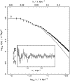
Matter power spectrum form measured from SDSS (Percival et al. 2007)

Fig. 13

Effect of wrong cosmological parameters on the power spectrum. The true one (solid line) assumes the cosmological parameters of Komatsu et al. (2011) (in particular ${\Omega }_{\mathrm{m}}=0.27$) and takes into account redshift space distortions. The wrong assumptions ${\Omega }_{\mathrm{m}}=0.3,0.5$ (dashed and dotted line, respectively) rescale the correlation function (on the left, multiplied by ${\theta }^2$ to enhance the BAOs) and the dimensionless power spectrum (on the right, divided by k to enhance the BAOs)

Fig. 14

Top panel: transverse (on the left) and radial (on the right) correlation function at $z=0.3,0.7,1,3$ from top to bottom, respectively. Bottom panel: the transverse power spectra at $z=0.1,0.5,1,3$ from top to bottom, respectively (on the left), and the radial one for $\ell =20$ and $z_1=1$ as function of $z_2$ (on the right). The standard, non-relativistic terms in blue, the relativistic corrections from lensing in magenta. Images reproduced with permission from [top] (Montanari and Durrer 2012), and [bottom] from Bonvin and Durrer (2011), copyright by APS

Fig. 15

Marginalized $\gamma -{\Sigma }_0$ forecast for weak lensing only analysis with Euclid. Here, ${\Sigma }_0$ is defined from $\Sigma =1+{\Sigma }_{0}a$ and $\Sigma$, defined via Eq. (I.3.28), is related to the WL potential. Black contours correspond to ${\ell }_{max}=5000$, demonstrating an error of 0.089$(1\sigma )$ on ${\Sigma }_0$, whereas the red contours correspond to ${\ell }_{max}=500$ giving an error of 0.034. In both cases, the inner and outer contours are $1\sigma$ and $2\sigma$ respectively. GR resides at [0.55, 0], while DGP resides at [0.68, 0]

Fig. 16

Constraints on $\gamma$, ${\alpha }_1$, ${\alpha }_2$ and A from Euclid, using a DGP fiducial model and 0.4 redshift bins between 0.3 and 1.5 for the central cosmological parameter values fitting $\text{WMAP}+\text{BAO}+\text{SNe}$

Fig. 17

Contour plots at 68 and 98% of probability for the pairs $s(z_i)-b(z_i)$ in 7 redshift bins (with $b=\sqrt{1+z}$). The ellipses are centered on the fiducial values of the growth rate and bias parameters, computed in the central values of the bins, $z_i$

Fig. 18

Expected constraints on the growth rates in each redshift bin. For each z the central error bars refer to the Reference case while those referring to the Optimistic and Pessimistic case have been shifted by $-0.015$ and $+0.015$ respectively. The growth rates for different models are also plotted: $\Lambda$CDM (green tight shortdashed curve), flat DGP (red longdashed curve) and a model with coupling between dark energy and dark matter (purple, dot-dashed curve). The blue curves (shortdashed, dotted and solid) represent the f(R) model by Hu and Sawicki (2007a), Eq. (I.5.36) with $n=0.5,1,2$ respectively and $\mu =3$. The plot shows that it will be possible to distinguish these models with next generation data

Fig. 19

Expected constraints on the growth rates in each redshift bin. For each z the central error bars refer to the Reference case while those referring to the Optimistic and Pessimistic case have been shifted by $-0.015$ and $+0.015$ respectively. The growth rates for different models are also plotted: $\Lambda$CDM (green tight shortdashed curve), flat DGP (red longdashed curve) and a model with coupling between dark energy and dark matter (purple, dot-dashed curve). Here we plot again the f(R) model by Hu and Sawicki (2007a), Eq. (I.5.36), with $n=2$ and $\mu =3$ (blue shortdashed curve) together with the model by Starobinsky (2007), Eq. (I.5.37), with $n=2$ and $\mu =3$ (cyan solid curve) and the one by Tsujikawa (2008), Eq. (I.5.38), with $\mu =1$ (black dotted curve). Also in this case it will be possible to distinguish these models with next generation data

Fig. 20

$\gamma$-parameterization. Left panel: 1 and 2$\sigma$ marginalized probability regions for constant $\gamma$ and w: the green (shaded) regions are relative to the Reference case, the blue long-dashed ellipses to the Optimistic case, while the black short-dashed ellipses are the probability regions for the Pessimistic case. The red dot marks the fiducial model; two alternative models are also indicated for comparison. Right panel: 1 and 2$\sigma$ marginalized probability regions for the parameters ${\gamma }_0$ and ${\gamma }_1$, relative to the Reference case (shaded yellow regions), to the Optimistic case (green long-dashed ellipses), and to the Pessimistic case (black dotted ellipses). Red dots represent the fiducial model, blue squares mark the DGP while triangles stand for the f(R) model. Then, in the case of $\gamma$-parameterization, one could distinguish these three models (at 95% probability)

Fig. 21

$\gamma$-parameterization. 1 and $2\sigma$ marginalized probability regions obtained assuming constant $\gamma$ and w (red solid curves) or assuming the parameterizations (I.8.5) and (I.8.2) and marginalizing over ${\gamma }_1$ and $w_1$ (black dashed curves); marginalized error values are in columns ${\sigma }_{{\gamma }_{\text{marg},1}}$, ${\sigma }_{w_{\text{marg},1}}$ of Table 8. Yellow dots represent the fiducial model, the triangles a f(R) model and the squares mark the flat DGP

Fig. 22

$\eta$-parameterization. 1 and 2$\sigma$ marginalized probability regions obtained assuming constant $\gamma$ and w (red solid curves) or assuming the parameterizations (I.8.6) and (I.8.2) and marginalizing over $\eta$ and $w_1$ (black dashed curves); marginalized error values are in columns ${\sigma }_{{\gamma }_{\text{marg},2}}$, ${\sigma }_{w_{\text{marg},2}}$ of Table 9. Yellow dots represent the fiducial model, the triangles stand for a f(R) model and the squares mark the flat DGP

Fig. 23

$\eta$-parameterization. Left panel: 1 and 2$\sigma$ marginalized probability regions for the parameters $\gamma$ and $\eta$ in Eq. (I.8.6) relative to the reference case (shaded blue regions), to the optimistic case (yellow long-dashed ellipses) and to the pessimistic case (black short-dashed ellipses). The red dot marks the fiducial model while the square represents the coupling model. Right panel: present constraints on $\gamma$ and $\eta$ computed through a full likelihood method (here the red dot marks the likelihood peak) (Di Porto and Amendola 2008)

Fig. 24

Errors on the equation of state. 1 and $2\sigma$ marginalized probability regions for the parameters $w_0$ and $w_1$, relative to the reference case and bias $b=\sqrt{(}1+z)$. The blue dashed ellipses are obtained fixing ${\gamma }_0,{\gamma }_1$ and ${\Omega }_k=0$ to their fiducial values and marginalizing over all the other parameters; for the red shaded ellipses instead, we also marginalize over ${\Omega }_k=0$ but we fix ${\gamma }_0,{\gamma }_1$. Finally, the black dotted ellipses are obtained marginalizing over all parameters but $w_0$ and $w_1$. The progressive increase in the number of parameters reflects in a widening of the ellipses with a consequent decrease in the figures of merit (see Table 11)

Fig. 25

Error bars on the Hubble parameter H(z) with five redshift bins. The exact height of the error bars respectively are (0.23, 0.072, 0.089, 0.064, 0.76)

Fig. 26

Error bars on the growth function G(z) with three redshift bins while marginalizing over the $h_i$s. The exact height of the error bars respectively are (0.029, 0.033, 0.25)

Fig. 27

Likelihood contours, for 65 and 95% C.L., calculated including signals up to $\ell \simeq 2000$ for the $\Lambda$CDM fiducial. Here simulations and halofit yield significantly different outputs

Fig. 28

On the left (right) panel, 1- and 2-$\sigma$ contours for the M1 (M3) model. The two fiducial models exhibit quite different behaviors

Fig. 29

Confidence region at 68% for three different values of $z_{max}=2.5,3.5,4$, red solid, green long-dashed and blue dashed contour, respectively. The left panel shows the confidence region when the sound speed is $c_s^2=1$; the right panel with the sound speed $c_s^2={10}^{-6}$. The equation of state parameter is for both cases $w_0=-0.8$

Fig. 30

Confidence region at 68% for three different values of $z_{max}=2.5,3.5,4$, red solid, green long-dashed and blue dashed contour, respectively. The left panel shows the confidence region when the sound speed is $c_s^2=1$; the right panel with the sound speed $c_s^2={10}^{-6}$. The equation of state parameter is for both cases $w_0=-0.8$

Fig. 31

The Bayes factor $lnB$ for the f(R) model of Eq. (I.5.36) over standard $\Lambda$CDM as a function of the extra parameter n. The green, red and blue curves refer to the conservative, bin-dependent and optimistic ${\ell }_{max}$, respectively. The horizontal lines denote the Jeffreys’ scale levels of significance

Fig. 32

Left panel: Linear matter power spectra for $\Lambda$CDM (solid line; $M_0^{-1}=0$, $\nu =1.5$) and scalaron (dashed line; $M_0^{-1}=375[{10}^{28}{\mathrm{h}}^{-1}{\mathrm{eV}}^{-1}]$, $\nu =1.5$) cosmologies. The modification to gravity causes a sizeable scale dependent effect in the growth of perturbations. The redshift dependence of the scalaron can be seen by comparing the top and bottom pairs of power spectra evaluated at redshifts $z=0.0$ and $z=1.5$, respectively. Right panel: The environmental dependent chameleon mechanism can be seen in the mildly nonlinear regime. We exhibit the fractional difference $(P(k)-P_{\mathrm{GR}}(k))/P_{\mathrm{GR}}(k)$ between the f(R) and GR power spectra for the model (I.8.37) with parameters $M_0^{-1}=375[{10}^{28}{\mathrm{h}}^{-1}{\mathrm{eV}}^{-1}]$ and $\nu =1.5$. The dashed lines represent linear power spectra (P(k) and $P_{\mathrm{GR}}(k)$ calculated with no higher order effects) and the solid lines are the power spectra calculated to second order. We see that the nonlinearities decrease the modified gravity signal. This is a result of the chameleon mechanism. The top set of lines correspond to $z=0$ and the bottom to $z=0.9$; demonstrating that the modified gravity signal dramatically decreases for larger z. This is due to the scalaron mass being much larger at higher redshifts. Furthermore, nonlinear effects are less significant for increasing z

Fig. 33

68% (dark grey) and 95% (light grey) projected bounds on the modified gravity parameters $M_0^{-1}$ and $\nu$ for the combined Euclid weak lensing and Planck CMB surveys. The larger (smaller) contours correspond to including modes $l=400(10,000)$ in the weak lensing analysis

Fig. 34

Comparison among predicted confidence contours for the cosmological parameter set $\Theta \equiv \{{\beta }^2,\alpha ,{\Omega }_c,h,{\Omega }_b,n_s,{\sigma }_8,log(A)\}$ using CMB (Planck, blue contours), P(k) (pink-violet contours) and weak lensing (orange-red contours) with Euclid-like specifications. Image reproduced by permission from Amendola et al. (2011), copyright by APS

Fig. 35

Redshift coverage and volume for the surveys mentioned in the text. Spectroscopic surveys only are shown. Recall that while future and forthcoming photometric surveys focus on weak gravitational lensing, spectroscopic surveys can extract the three dimensional galaxy clustering information and therefore measure radial and tangential BAO signal, the power spectrum shape and the growth of structure via redshift space distortions. The three-dimensional clustering information is crucial for BAO. For example to obtain the same figure of merit for dark-energy properties a photometric survey must cover a volume roughly ten times bigger than a spectroscopic one

Fig. 36

We show the figure of merit for ${\omega }_{\mathit{CDM}}=h^2{\Omega }_{\mathit{CDM}}$ and $H_0$ as a function of the number of bins for the photometric survey of Euclid. The black line is the P(k) result, the red dashed line is the $C_l(z_1,z_2)$ result for bin auto-correlations only, while the blue line also includes cross-correlations

Fig. 37

The baryonic mass function of galaxies (data points). The dotted line shows a Schechter function fit to the data. The blue line shows the predicted mass function of dark matter haloes, assuming that dark matter is cold. The red line shows the same assuming that dark matter is warm with a (thermal relic) mass of $m_{\mathrm{WDM}}=1\mathrm{keV}$

Fig. 38

The fraction of mass in bound structures as a function of redshift, normalized to a halo of Milky Way’s mass at redshift $z=0$. Marked are different masses of thermal-relic WDM particles in keV (black solid lines). Notice that the differences between different WDM models increases towards higher redshift

Fig. 39

The central log-slope $\alpha$ of the density distribution $\rho \propto r^{\alpha }$ for 9 galaxies/groups and 3 lensing clusters as a function of the enclosed lensing mass. Marked in red is the prediction from structure formation simulations of the standard cosmological model, that assume non-relativistic CDM, and that do not include any baryonic matter

Fig. 40

Full hydrodynamical simulations of massive clusters at redshift $z=0.6$. Total projected mass is shown in blue, while X-ray emission from baryonic gas is in red. The preferential trailing of gas due to pressure from the ICM, and its consequent separation from the non interacting dark matter, is apparent in much of the infalling substructure

Fig. 41

Constraints from neutrino oscillations and from cosmology in the m–$\Sigma$ plane. Image reproduced by permission from Jiménez et al. (2010); copyright by IOP and SISSA

Fig. 42

Left: region in the $\Delta$–$\Sigma$ parameter space allowed by oscillations data. Right: Weak lensing forecasts. The dashed and dotted vertical lines correspond to the central value for $\Delta$ given by oscillations data. In this case Euclid could discriminate NI from IH with a $\Delta {\chi }^2=2$. Image reproduced by permission from Jiménez et al. (2010); copyright by IOP and SISSA

Fig. 43

DM halo mass function (MF) as a function of $\Sigma$ and redshift. MF of the SUBFIND haloes in the $\Lambda$CDM N-body simulation (blue circles) and in the two simulations with $\Sigma =0.3\mathrm{eV}$ (magenta triangles) and $\Sigma =0.6\mathrm{eV}$ (red squares). The blue, magenta and red lines show the halo MF predicted by Sheth and Tormen (2002), where the variance in the density fluctuation field, $\sigma (M)$, at the three cosmologies, $\Sigma =0,0.3,0.6\mathrm{eV}$, has been computed with the software camb (Lewis et al. 2000b)

Fig. 44

Real space two-point auto-correlation function of the DM haloes in the $\Lambda$CDM N-body simulation (blue circles) and in the simulation with $\Sigma =0.6\mathrm{eV}$ (red squares). The blue and red lines show the DM correlation function computed using the camb matter power spectrum with $\Sigma =0$ and $\Sigma =0.6\mathrm{eV}$, respectively. The bottom panels show the ratio between the halo correlation function extracted from the simulations with and without massive neutrinos

Fig. 45

Bias of the DM haloes in the $\Lambda$CDM N-body simulation (blue circles) and in the two simulations with $\Sigma =0.3\mathrm{eV}$ (magenta triangles) and $\Sigma =0.6\mathrm{eV}$ (red squares). Dotted lines are the theoretical predictions of Sheth et al. (2001)

Fig. 46

Mean bias (averaged in $10<r[\mathrm{Mpc}/h]<50$) as a function of redshift compared with the theoretical predictions of Sheth and Tormen (2002). Here the dashed lines represent the theoretical expectations for a $\Lambda$CDM cosmology renormalized with the ${\sigma }_8$ value of the simulations with a massive neutrino component

Fig. 47

Two-point auto-correlation function in real and redshift space of the DM haloes in the $\Lambda$CDM N-body simulation (blue circles) and in the simulation with $\Sigma =0.6\mathrm{eV}$ (red squares). The bottom panels show the ratio between them, compared with the theoretical expectation

Fig. 48

Best-fit values of $\beta$-${\sigma }_{12}$, as a function of $\Sigma$ and redshift (points), compared with the theoretical prediction (grey shaded area). The blue dotted lines show the theoretical prediction for a $\Lambda$CDM cosmology normalised to the ${\sigma }_8$ value of the simulation with a massive neutrino component

Fig. 49

The $z=0$ matter power spectrum arising in UDM models with a Lagrangian given by Eq. (II.9.4). $\Lambda$CDM is solid, and UDM models with $c_{\infty }={10}^{-1},{10}^{-2},{10}^{-3}$ are shown from bottom to top. Image reproduced by permission from Camera et al. (2011c), copyright by the authors

Fig. 50

Marginalized uncertainty in $f_{\mathit{ax}}$ for CMB (green), a galaxy redshift survey (red), weak lensing (blue) and the total (black) evaluated for four different fiducial axion masses, for the cosmology $\Lambda \text{CDM}+f_{\mathit{ax}}+\nu$. Image reproduced by permission from Marsh et al. (2012), copyright by APS

Fig. 51

Mapping between axion and WDM mass that suppress power by a factor of two at the same scale. This can be used to approximately the axion mass constraint possible with Euclid on based on WDM forecasts

Fig. 52

The marginalized likelihood contours (68.3 and 95.4% CL) for Planck forecast only (blue dashed lines) and Planck plus Euclid pessimistic (red filled contours). The white points correspond to the fiducial model

Fig. 53

For illustration purposes this is the effect of a local $f_{\mathrm{NL}}$ of $\pm 50$ on the $z=0$ power spectrum of halos with mass above ${10}^{13}{M}_{\odot }$

Fig. 54

Constraints on possible violation of the Etherington relation in the form of deviations from a perfectly transparent universe ($ϵ=0$). The corresponding constraint on the parameter $\beta$, quantifying violations from the standard temperature-redshift relation, can be read in the upper x-axis. Blue regions represent current constraints while orange are forecast Euclid constraints assuming it is accompanied by a Dark Energy Task Force stage IV supernovae sample. Image reproduced with permission from Avgoustidis et al. (2010), copyright by IOP

Fig. 55

Forecasted 68 and 95% likelihood contours for SN (filled blue), H(z) (dashed line transparent) and combined SN+H(z) (solid line transparent), assuming Euclid BAO is accompanied by a SNAP-like (or Dark Energy Task Force stage IV) supernova sample. We show constraints on the ${\Omega }_m-w$ plane, having marginalised over all other parameters in the context of flat wCDM models. On the left, we have allowed a coupling between photons and a putative dark energy scalar at the level allowed by current data, while on the right we have set this coupling to zero. The dotted contours on the left show SN contours assuming constraints on this coupling can be improved by an order of magnitude. Note how the joint contours become dominated by the SN data if this coupling is strongly constrained

Fig. 56

Constraints on the simplest Axion-like particles models. Blue regions represent current constraints while orange are forecast Euclid constraints assuming it is accompanied by a Dark Energy Task Force stage IV supernovae sample. Here P / L is the conversion probability per unit length and is the relevant parameter for $\tau (z)$. Image reproduced with permission from Avgoustidis et al. (2010), copyright by IOP

Fig. 57

Constraints on MCP models. Blue regions represent current constraints while orange are forecast Euclid constraints assuming it is accompanied by a Dark Energy Task Force stage IV supernovae sample. Image reproduced with permission from Avgoustidis et al. (2010), copyright by IOP

Fig. 58

Marginalized constraints on the amount of radial inhomogeneity ${\delta }_0$ at a given scale L from local Hubble parameter measurements, supernova Ia data, CMB anisotropies, BAO observations, Compton y-distortion and kSZ constraints and age data (as lower bounds only) at 68, 95 and 99% confidence level (blue contours), compared to the expected level of inhomogeneity within a $\Lambda$CDM model that satisfies the Copernican principle (red-to-gray contours). Image reproduced with permission from Valkenburg et al. (2013b), copyright by the authors

Fig. 59

Relative errors on ${\Omega }_K$ for our benchmark survey for different redshifts

Fig. 60

Left: same as Fig. 59 but now with superimposed the prediction for the Lemaître–Tolman–Bondi model considered by García-Bellido and Haugbølle (2008a). Right: zoom in the high-redshift range

Fig. 61

Supernova and CMB constraints in the $({\Omega }_m^{{\mathcal{D}}_0},n)$ plane for the averaged effective model with zero Friedmannian curvature (filled ellipses) and for a standard flat FLRW model with a quintessence field with constant equation of state $w=-(n+3)/3$ (black ellipses). The disk and diamond represent the absolute best-fit models respectively for the standard FLRW model and the averaged effective model

Fig. 62

Projected cosmological 8-parameter space for a 15,000 square degrees, median redshift of $z=0.8$, 10 bin tomographic cosmic shear survey. Specifications are based on Euclid Yellow book (Laureijs et al. 2009) as this figure is representative of a method, rather than on forecast analysis; the discussion is still valid with more updated (Laureijs et al. 2011) Euclid specifications. The upper panel shows the 1D parameter constraints using analytic marginalization (black) and the Gaussian approximation (Fisher matrix, blue, dark grey). The other panels show the 2D parameter constraints. Grey contours are 1- 2- and 3-$\sigma$ levels using analytic marginalization over the extra parameters, solid blue ellipses are the 1-$\sigma$ contours using the Fisher-matrix approximation to the projected likelihood surface, solid red ellipses are the 1-$\sigma$ fully marginalized. Image reproduced by permission from Taylor and Kitching (2010)

Fig. 63

Gaussian approximation (Laplace approximation) to a 6-dimensional posterior distribution for cosmological parameters, from WMAP1 and SDSS data. For all couples of parameters, panels show contours enclosing 68 and 95% of joint probability from $2\times {10}^5$ MC samples (black contours), along with the Laplace approximation (red ellipses). It is clear that the Laplace approximation captures the bulk of the posterior volume in parameter space in this case where there is little non-Gaussianity in the posterior PDF. Image reproduced from 2005 preprint of Trotta (2007a)

References

1. Abazajian K, Switzer ER, Dodelson S, Heitmann K, Habib S. Nonlinear cosmological matter power spectrum with massive neutrinos: the halo model. Phys Rev D. 2005;71:043507. doi: 10.1103/PhysRevD.71.043507. - DOI
1. Abazajian KN, Acero MA, Agarwalla SK, Aguilar-Arevalo AA, Albright CH et al (2012b) Light sterile neutrinos: a white paper. ArXiv e-prints 1204.5379
1. Abbott LF, Sikivie P. A cosmological bound on the invisible axion. Phys Lett B. 1983;120:133–136. doi: 10.1016/0370-2693(83)90638-X. - DOI
1. Abbott BP, et al. Observation of gravitational waves from a binary black hole merger. Phys Rev Lett. 2016;116:061102. doi: 10.1103/PhysRevLett.116.061102. - DOI - PubMed
1. Abdalla E, Abramo LR, Sodré L, Jr, Wang B. Signature of the interaction between dark energy and dark matter in galaxy clusters. Phys Lett B. 2009;673:107–110. doi: 10.1016/j.physletb.2009.02.008. - DOI