Computational mechanisms underlying cortical responses to the affordance properties of visual scenes

Abstract

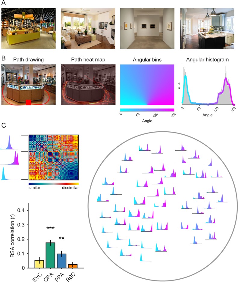
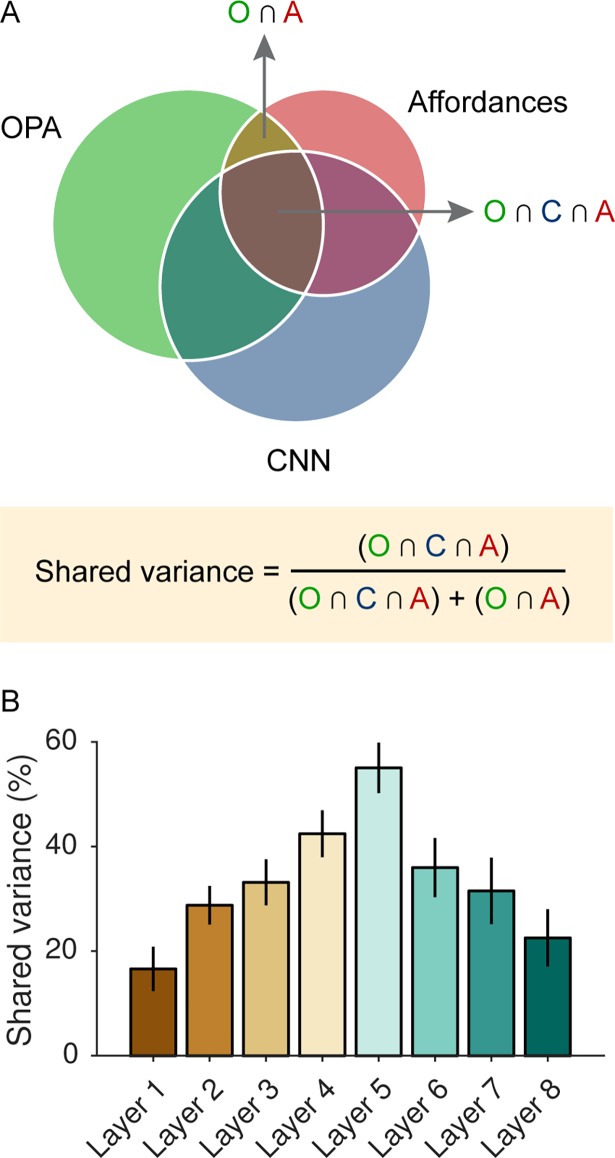
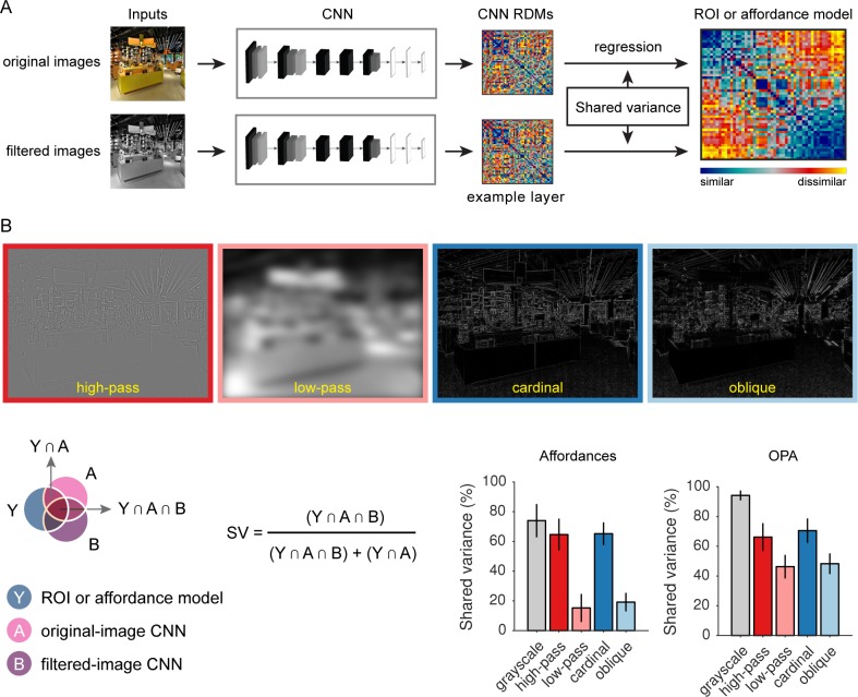
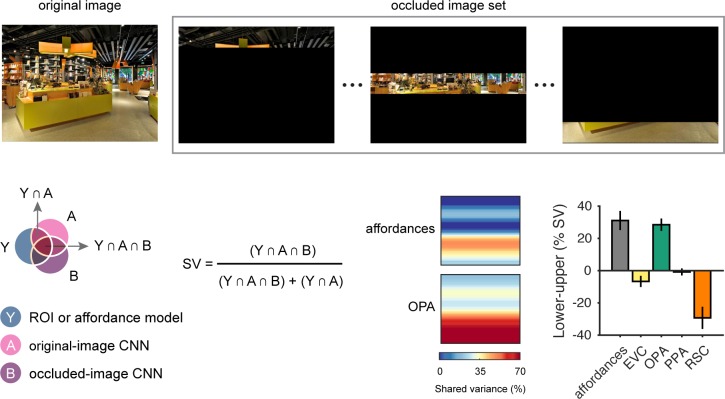
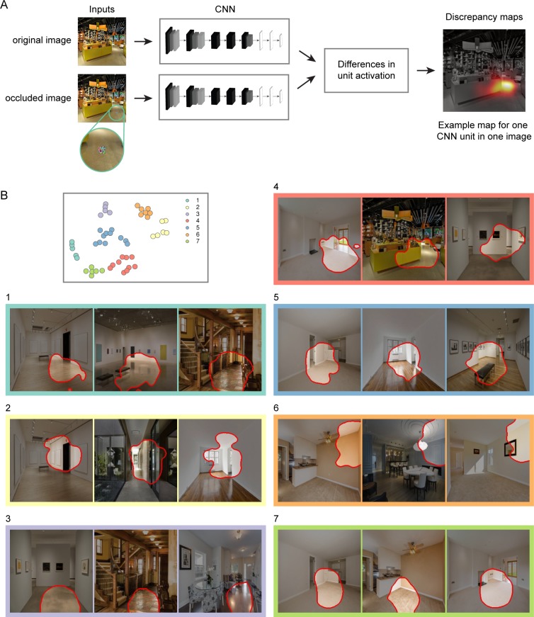
Biologically inspired deep convolutional neural networks (CNNs), trained for computer vision tasks, have been found to predict cortical responses with remarkable accuracy. However, the internal operations of these models remain poorly understood, and the factors that account for their success are unknown. Here we develop a set of techniques for using CNNs to gain insights into the computational mechanisms underlying cortical responses. We focused on responses in the occipital place area (OPA), a scene-selective region of dorsal occipitoparietal cortex. In a previous study, we showed that fMRI activation patterns in the OPA contain information about the navigational affordances of scenes; that is, information about where one can and cannot move within the immediate environment. We hypothesized that this affordance information could be extracted using a set of purely feedforward computations. To test this idea, we examined a deep CNN with a feedforward architecture that had been previously trained for scene classification. We found that responses in the CNN to scene images were highly predictive of fMRI responses in the OPA. Moreover the CNN accounted for the portion of OPA variance relating to the navigational affordances of scenes. The CNN could thus serve as an image-computable candidate model of affordance-related responses in the OPA. We then ran a series of in silico experiments on this model to gain insights into its internal operations. These analyses showed that the computation of affordance-related features relied heavily on visual information at high-spatial frequencies and cardinal orientations, both of which have previously been identified as low-level stimulus preferences of scene-selective visual cortex. These computations also exhibited a strong preference for information in the lower visual field, which is consistent with known retinotopic biases in the OPA. Visualizations of feature selectivity within the CNN suggested that affordance-based responses encoded features that define the layout of the spatial environment, such as boundary-defining junctions and large extended surfaces. Together, these results map the sensory functions of the OPA onto a fully quantitative model that provides insights into its visual computations. More broadly, they advance integrative techniques for understanding visual cortex across multiple level of analysis: from the identification of cortical sensory functions to the modeling of their underlying algorithms.

Fig 1. Navigational-affordance information is coded in scene-selective visual cortex.

(A) Examples of natural images used in the fMRI experiment. All experimental stimuli were images of indoor environments with clear navigational paths proceeding from the bottom center of the image. (B) In a norming study, an independent group of raters indicated with a computer mouse the paths that they would take to walk through each scene, starting from the red square at the bottom center of the image (far left panel). These data were combined across subjects to create heat maps of the navigational paths in each image (middle left panel). We summed the values in these maps along one-degree angular bins radiating from the bottom center of the image (middle right panel), which produced histograms of navigational probability measurements over a range of angular directions (far right panel). The gray bars in this histogram represent raw data, and the overlaid line indicates the angular data after smoothing. (C) The navigational histograms were compared pairwise across all images to create a model RDM of navigational-affordance coding (top left panel). Right panel shows a two-dimensional visualization of this representational model, created using t-distributed stochastic neighbor embedding (t-SNE), in which the navigational histograms for each condition are plotted within the two-dimensional embedding. RSA correlations were calculated between the model RDM and neural RDMs for each ROI (bottom left panel). The strongest RSA effect for the coding of navigational affordances was in the OPA. There was also a significant effect in the PPA. Error bars represent bootstrap ±1 s.e.m. a.u. = arbitrary units. **p<0.01, ***p<0.001.

Fig 2. Navigational-affordance information can be extracted by a feedforward computational model.

(A) Architecture of a deep CNN trained for scene categorization. Image pixel values are passed to a feedforward network that performs a series of linear-nonlinear operations, including convolution, rectified linear activation, local max pooling, and local normalization. The final layer contains category-detector units that can be interpreted as signaling the association of the image with a set of semantic labels. (B) RSA of the navigational-affordance model and the outputs from each layer of the CNN. The affordance model correlated with multiple layers of the CNN, with the strongest effects observed in higher convolutional layers and weak or no effects observed in the earliest layers. This is consistent with the findings of the fMRI experiment, which indicate that navigational affordances are coded in mid-to-high-level visual regions but not early visual cortex. (C) RSA of responses in the OPA and the outputs from each layer of the CNN. All layers showed strong RSA correlations with the OPA, and the peak correlation was in layer 5, the highest convolutional layer. Error bars represent bootstrap ±1 s.e.m. *p<0.05, **p<0.01.

Fig 3. The CNN accounts for shared variance between OPA responses and the navigational-affordance model.

(A) A variance-partitioning procedure, known as commonality analysis, was used to quantify the portion of the shared variance between the OPA RDM and the navigational-affordance RDM that could be accounted for by the CNN. Commonality analysis partitions the explained variance of a multiple regression model into the unique and shared variance contributed by all of its predictors. In this case, multiple regression RSA was performed with the OPA as the predictand and the affordance and CNN models as predictors. (B) Partitioning the explained variance of the affordance and CNN models showed that over half of the variance explained by the navigational-affordance model in the OPA could be accounted for by the highest convolutional layer of the CNN (layer 5). Error bars represent bootstrap ±1 s.e.m.

Fig 4. Analysis of low-level image features that underlie the predictive accuracy of the CNN.

(A) Experiments were run on the CNN to quantify the contribution of specific low-level image features to the representational similarity between the CNN and the OPA and between the CNN and the navigational-affordance model. First, the original stimuli were passed through the CNN, and RDMs were created for each layer. Then the stimuli were filtered to isolate or remove specific visual features. For example, grayscale images were created to remove color information. These filtered stimuli were passed through the CNN, and new RDMs were created for each layer. Multiple-regression RSA was performed using the RDMs for the original and filtered stimuli as predictors. Commonality analysis was applied to this regression model to quantify the portion of the shared variance between the CNN RDM and the OPA RDM or between the CNN RDM and the affordance RDM that could be accounted for by the filtered stimuli. (B) This procedure was used to quantify the contribution of color (grayscale), spatial frequencies (high-pass and low-pass), and edge orientations (cardinal and oblique). The RSA effects of the CNN were driven most strongly by grayscale information at high spatial frequencies and cardinal orientations. Over half of the shared variance between the CNN and the OPA and between the CNN and the affordance model could be accounted for by representations of grayscale images or images containing only high-spatial frequency information or edges at cardinal orientations. In contrast, the contributions of low spatial frequencies and edges at oblique orientations were considerably lower. These differences in high-versus-low spatial frequencies and cardinal-versus-oblique orientations were more pronounced for RSA predictions of the navigational-affordance RDM, but a similar pattern was observed for the OPA RDM. Bars represent means and error bars represent ±1 s.e.m. across CNN layers.

Fig 5. Visual-field biases in the predictive accuracy of the CNN.

Experiments were run on the CNN to quantify the importance of visual inputs at different positions along the vertical axis of the image. First, the original stimuli were passed through the CNN, and RDMs were created. Then the stimuli were occluded to mask everything outside of a small horizontal slice of the image (top panel). These occluded stimuli were passed through the CNN, and new RDMs were created. Multiple regression RSA was performed using the RDMs for the original and occluded images as predictors. Commonality analysis was applied to this regression model to quantify the portion of the shared variance between the CNN and the OPA or between the CNN and the navigational-affordance model that could be accounted for by the occluded images (bottom left panel). This procedure was repeated with the un-occluded region slightly shifted on each iteration until the entire vertical axis of the image was sampled. Results indicated that the RSA effects of the CNN were driven most strongly by features in the lower half of the image (bottom right panel). This effect was most pronounced for RSA predictions of the OPA RDM, in which ~70% of the explained variance of the CNN could be accounted for by visual information within a small slice of the image from the lower visual field. A summary statistic of this visual-field bias, created by calculating the difference in mean shared variance across the lower and upper halves of the image, showed that a bias for information in the lower visual field was observed for the affordance model and the OPA, but not for EVC, PPA, or RSC. Bars represent means and error bars represent ±1 s.e.m. across CNN layers.

Fig 6. Receptive-field selectivity of CNN units.

(A) The selectivity of individual CNN units was mapped across each image through an iterative occlusion procedure. First, the original image was passed through the CNN. Then a small portion of the image was occluded with a patch of random pixel values. The occluded image was passed though the CNN, and the discrepancies in unit activations relative to the original image were logged. After iteratively applying this procedure across all spatial positions in the image, a two-dimensional discrepancy map was generated for each CNN unit and each stimulus (far right panel). Each discrepancy map indicates the sensitivity of a CNN unit to the visual information within an image. The two-dimensional position of its peak effect reflects the unit’s spatial receptive field, and the magnitude of its peak effect reflects the unit’s selectivity for the image features within this receptive field. (B) Receptive-field visualizations were generated for a subset of the units in layer 5 that had strong unit-wise RSA correlations with the OPA and the affordance model. To examine the visual motifs detected by these units, we created a two-dimensional embedding of the units based on the visual similarity of the image features that drove their responses. A clustering algorithm was then used to identify groups of units whose responses reflect similar visual motifs (top left panel). This data-driven procedure identified 7 clusters, which are color-coded and numbered in the two-dimensional embedding. Visualizations are shown for an example unit from each cluster (the complete set of visualizations can be seen in S1–S7 Figs). These visualizations were created by identifying the top 3 images with the largest discrepancy values in the receptive-field mapping procedure (i.e., images that were strongly representative of a unit’s preferences). A segmentation mask was then applied to each image by thresholding the unit’s discrepancy map at 10% of the peak discrepancy value. Segmentations highlight the portion of the image that the unit was sensitive to. Each segmentation is outlined in red, and regions of the image outside of the segmentation are darkened. Among these visualizations, two broad themes were discernable: boundary-defining junctions (e.g., clusters 1, 5, 6, and 7) and large extended surfaces (e.g., cluster 3). The boundary-defining junctions included junctions where two or more large planes meet (e.g., a wall and a floor). Large extended surfaces included uninterrupted portions of floor and wall planes. There were also units that detected features indicative of doorways and other open pathways (e.g., clusters 2 and 4). All of these high-level features appear to be well-suited for mapping out the spatial layout and navigational boundaries in a visual scene.

Fig 7. Classification of navigability in natural landscapes.

(A) Units from layer 5 of the CNN were used to classify navigability and other scene properties in a set of natural outdoor scenes. Classifier performance was examined for a subset of units that were strongly associated with navigational-affordance representation in our previous analyses of indoor scenes. Specifically, a classifier was created from the 50 units in layer 5 that were selected for the visualization analyses in Fig 6. For comparison, a resampling distribution was generated by randomly selecting 50 units from layer 5 over 5,000 iterations and submitting these units to the same classification procedures. Classification accuracy was quantified through leave-one-out cross-validation. For each scene property, the label for a given image was predicted from a linear classifier trained on all other images. This procedure was repeated for each image in turn, and accuracy was calculated as the percentage of correct classifications across all images. In this plot, the black dots indicate the classification accuracies obtained from the 50 affordance-related CNN units, and the shaded kernel density plots indicate the accuracy distributions obtained from randomly resampled units. Each kernel density distribution was mirrored across the vertical axis, with the area in between shaded gray. These analyses showed that the strongly affordance-related units performed at 90% accuracy when classifying natural landscapes based on navigation (i.e., overall navigability). This accuracy was in the 99th percentile of the resampling distribution, suggesting that these units were particularly informative for identifying scene navigability. Furthermore, these units were more accurate at classifying navigation than any other scene property. (B) Examples of images that were correctly classified into the categories of low or high navigability based on the responses of the affordance-related units. These images illustrate some of the high-level scene features that influenced overall navigability, including spatial layout, textures, and material properties. (C) All images that were misclassified into categories of low or high navigability based on the responses of the affordance-related units. The label above each image is the incorrect label produced by the classifier. Many of the misclassified images contain materials on the ground plane that were uncommon in this stimulus set.

References

1. LeCun Y, Bengio Y, Hinton G. Deep learning. Nature. 2015;521(7553):436–44. doi: 10.1038/nature14539 - DOI - PubMed
1. Krizhevsky A, Sutskever I, Hinton GE. Imagenet classification with deep convolutional neural networks. Advances in neural information processing systems 2012. p. 1097–105.
1. Zhou B, Lapedriza A, Xiao J, Torralba A, Oliva A. Learning deep features for scene recognition using places database. Advances in neural information processing systems 2014. p. 487–95.
1. Rawat W, Wang Z. Deep convolutional neural networks for image classification: a comprehensive review. Neural Comput. 2017. Epub June 09, 2017. doi: 10.1162/NECO_a_00990 . - DOI - PubMed
1. Agrawal P, Stansbury D, Malik J, Gallant JL. Pixels to voxels: modeling visual representation in the human brain. arXiv preprint arXiv:14075104. 2014.
Publication types
LinkOut - more resources