A Dynamic Connectome Supports the Emergence of Stable Computational Function of Neural Circuits through Reward-Based Learning

Abstract

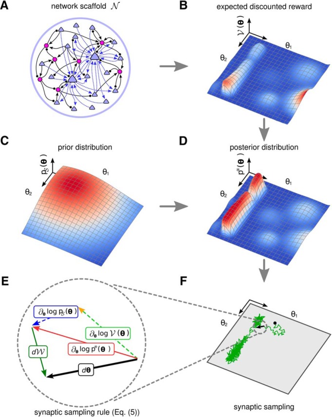
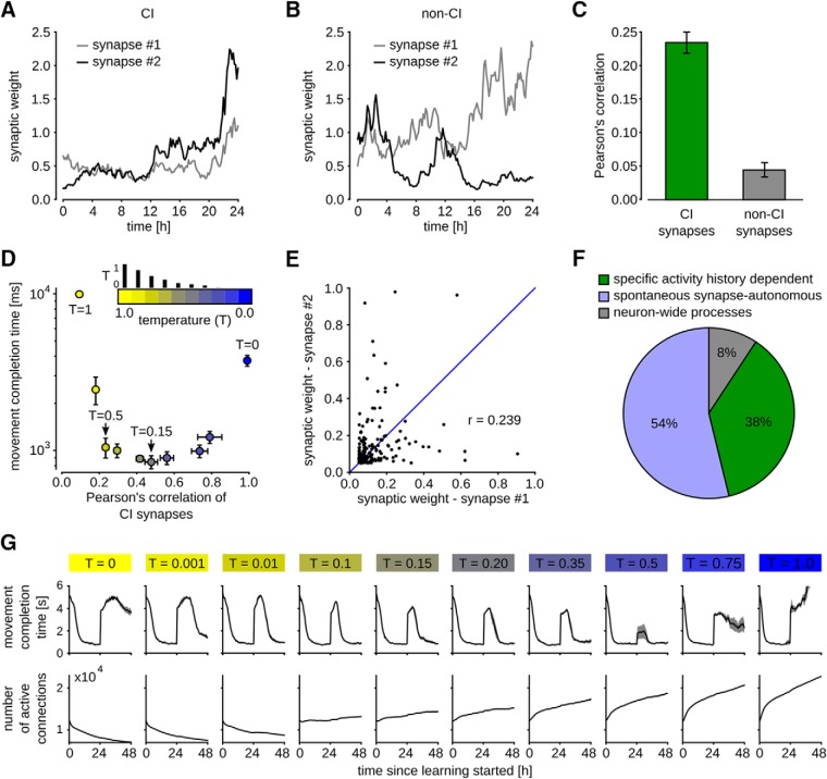
Synaptic connections between neurons in the brain are dynamic because of continuously ongoing spine dynamics, axonal sprouting, and other processes. In fact, it was recently shown that the spontaneous synapse-autonomous component of spine dynamics is at least as large as the component that depends on the history of pre- and postsynaptic neural activity. These data are inconsistent with common models for network plasticity and raise the following questions: how can neural circuits maintain a stable computational function in spite of these continuously ongoing processes, and what could be functional uses of these ongoing processes? Here, we present a rigorous theoretical framework for these seemingly stochastic spine dynamics and rewiring processes in the context of reward-based learning tasks. We show that spontaneous synapse-autonomous processes, in combination with reward signals such as dopamine, can explain the capability of networks of neurons in the brain to configure themselves for specific computational tasks, and to compensate automatically for later changes in the network or task. Furthermore, we show theoretically and through computer simulations that stable computational performance is compatible with continuously ongoing synapse-autonomous changes. After reaching good computational performance it causes primarily a slow drift of network architecture and dynamics in task-irrelevant dimensions, as observed for neural activity in motor cortex and other areas. On the more abstract level of reinforcement learning the resulting model gives rise to an understanding of reward-driven network plasticity as continuous sampling of network configurations.

Keywords: reward-modulated STDP; spine dynamics; stochastic synaptic plasticity; synapse-autonomous processes; synaptic rewiring; task-irrelevant dimensions in motor control.

Graphical abstract

Figure 1.

Illustration of the theoretical framework. A, A neural network scaffold $\mathrm{N}$ of excitatory (blue triangles) and inhibitory (purple circles) neurons. Potential synaptic connections (dashed blue arrows) of only two excitatory neurons are shown to keep the figure uncluttered. Synaptic connections (black connections) from and to inhibitory neurons are assumed to be fixed for simplicity. B, A reward landscape for two parameters $\mathit{\text{θ}}=\{{\theta }_1,{\theta }_2\}$ with several local optima. Z-amplitude and color indicate the expected reward $\mathrm{V}(\mathit{\text{θ}})$ for given parameters $\mathit{\text{θ}}$ (X-Y plane). C, Example prior that prefers small values for θ₁ and θ₂. D, The posterior distribution $p^{*}(\mathit{\text{θ}})$ that results as product of the prior from C and the expected discounted reward of B. E, Illustration of the dynamic forces (plasticity rule Eq. 5) that act on $\mathit{\text{θ}}$ in each sampling step $d\mathit{\text{θ}}$ (black) while sampling from the posterior distribution. The deterministic term (red), which consists of the first two terms (prior and reward expectation) in Equation 5, is directed to the next local maximum of the posterior. The stochastic term $d\mathcal{W}$ (green) of Equation 5 has a random direction. F, A single trajectory of policy sampling from the posterior distribution of D under Equation 5, starting at the black dot. The parameter vector $\mathit{\text{θ}}$ fluctuates between different solutions and moves primarily along the task-irrelevant dimension θ₂.

Figure 2.

Reward-based routing of input patterns. A, Illustration of the network scaffold. A population of 20 model MSNs (blue) receives input from 200 excitatory input neurons (green) that model cortical neurons. Potential synaptic connections between these two populations of neurons were subject to reward-based synaptic sampling. In addition, fixed lateral connections provided recurrent inhibitory input to the MSNs. The MSNs were divided into two groups, each projecting exclusively to one of two target areas T₁ and T₂. Reward was delivered whenever the network managed to route an input pattern P_i primarily to that group of MSNs that projected to target area T_i. B, Illustration of the model for spine dynamics. Five potential synaptic connections at different states are shown. Synaptic spines are represented by circular volumes with diameters proportional to $\sqrt[3]{{\mathit{w}}_i}$ for functional connections, assuming a linear correlation between spine-head volume and synaptic efficacy w_i (Matsuzaki et al., 2001). C, Dynamics of weights w_i in log scale for 10 potential synaptic connections i when the activity-dependent term $\frac{\partial }{\partial {\theta }_i}\log \mathrm{V}(\mathit{\text{θ}})dt$ in Equation 5 is set equal to zero). As in experimental data (Holtmaat et al., 2006, their Fig. 2I) the dynamics is in this case consistent with an Ornstein–Uhlenbeck process in the logarithmic scale. Weight values are plotted relative to the initial value at time 0. D, E, Dynamics of a model synapse when a reward-modulated STDP pairing protocol as in Yagishita et al. (2014) was applied. D, Reward delivery after repeated firing of the presynaptic neuron before the postsynaptic neuron resulted in a strong weight increase (left). This effect was reduced without reward (right) and prevented completely if no presynaptic stimulus was applied. Values in D, E represent percentage of weight changes relative to the pairing onset time (dashed line, means ± SEM over 50 synapses). Compare with Yagishita et al. (2014), their Figure 1F,G. E, Dependence of resulting changes in synaptic weights in our model as a function of the delay of reward delivery. Gray shaded rectangle indicates the time window of STDP pairing application. Reward delays denote time between paring and reward onset. Compare to Yagishita et al. (2014), their Figure 1O. F, The average reward achieved by the network increased quickly during learning according to Equation 5 (mean over five independent trial runs; shaded area indicates SEM). G, Synaptic parameters kept changing throughout the experiment in F. The magnitude of the change of the synaptic parameter vector $\mathit{\text{θ}}$ is shown (mean ± SEM as in F; Euclidean norm, normalized to the maximum value). The parameter change peaks at the onset of learning but remains high (larger than 80% of the maximum value) even when stable performance has been reached. H, Spiking activity of the network during learning. Activities of 20 randomly selected input neurons and all MSNs are shown. Three salient input neurons (belonging to pools S₁ or S₂ in I) are highlighted. Most neurons have learnt to fire at a higher rate for the input pattern P_j that corresponds to the target area T_j to which they are projecting. Bottom, Reward delivered to the network. I, Dynamics of network rewiring throughout learning. Snapshots of network configurations for the times t indicated below the plots are shown. Gray lines indicate active connections between neurons; connections that were not present at the preceding snapshot are highlighted in green. All output neurons and two subsets of input neurons that fire strongly in pattern P₁ or P₂ are shown (pools S₁ and S₂, 20 neurons each). Numbers denote total counts of functional connections between pools. The connectivity was initially dense and then rapidly restructured and became sparser. Rewiring took place all the time throughout learning. J, Analysis of random exploration in task-irrelevant dimensions of the parameter space. Projection of the parameter vector $\mathit{\text{θ}}$ to the two dPCA components that best explain the variance of the average reward. dpc1 explains >99.9% of the reward variance (dpc2 and higher dimensions <0.1%). A single trajectory of the high-dimensional synaptic parameter vector over 24 h of learning projected onto dpc1 and dpc2 is shown. Amplitude on the y-axis denotes the estimated average reward (in fractions of the total maximum achievable reward). After converging to a region of high reward (movement mainly along dpc1), network continues to explore task-irrelevant dimensions (movement mainly along dpc2).

Figure 3.

Reward-based self-configuration and compensation capability of a recurrent neural network. A, Network scaffold and task schematic. Symbol convention as in Figure 1A. A recurrent network scaffold of excitatory and inhibitory neurons (large blue circle); a subset of excitatory neurons received input from afferent excitatory neurons (indicated by green shading). From the remaining excitatory neurons, two pools D and U were randomly selected to control lever movement (blue shaded areas). Bottom inset, Stereotypical movement that had to be generated to receive a reward. B, Spiking activity of the network at learning onset and after 22 h of learning. Activities of random subsets of neurons from all populations are shown (hidden: excitatory neurons of the recurrent network, which are not in pool D or U). Bottom, Lever position inferred from the neural activity in pools D and U. Rewards are indicated by red bars. Gray shaded areas indicate cue presentation. C, Task performance quantified by the average time from cue presentation onset to movement completion. The network was able to solve this task in <1 s on average after ∼8 h of learning. A task change was introduced at time 24 h (asterisk; function of D and U switched), which was quickly compensated by the network. Using a simplified version of the learning rule, where the reintroduction of nonfunctional potential connections was approximated using exponentially distributed waiting times (green), yielded similar results (see also E). If the connectome was kept fixed after the task change at 24 h, performance was significantly worse (black). D, Trial-averaged network activity (top) and lever movements (bottom). Activity traces are aligned to movement onsets (arrows); y-axis of trial-averaged activity plots are sorted by the time of highest firing rate within the movement at various times during learning: sorting of the first and second plot is based on the activity at t = 0 h, third and fourth by that at t = 22 h, fifth is resorted by the activity at t = 46 h. Network activity is clearly restructured through learning with particularly stereotypical assemblies for sharp upward movements. Bottom: average lever movement (black) and 10 individual movements (gray). E, Turnover of synaptic connections for the experiment shown in D; y-axis is clipped at 3,000. Turnover rate during the first 2 h was around 12,000 synapses (∼25%) and then decreased rapidly. Another increase in spine turnover rate can be observed after the task change at time 24 h. F, Effect of forgetting due to parameter diffusion over 14 simulated days. Application of reward was stopped after 24 h when the network had learned to reliably solve the task. Parameters subsequently continue to evolve according to the SDE (Eq. 5). Onset of forgetting can be observed after day 6. A simple consolidation mechanism triggered after 4 days reliably prevents forgetting. G, Histograms of time intervals between disappearance and reappearance of synapses (waiting times) for the exact (upper plot) and approximate (lower plot) learning rule. H, Relative fraction of potential synaptic connections that were stably nonfunctional, transiently decaying, transiently emerging or stably function during the relearning phase for the experiment shown in D. I, PCA of a random subset of the parameters θ_i. The plot suggests continuing dynamics in task-irrelevant dimensions after the learning goal has been reached (indicated by red color). When the function of the neuron pools U and D was switched after 24 h, the synaptic parameters migrated to a new region. All plots show means over five independent runs (error bars: SEM).

Figure 4.

Impact of the prior distribution and reward amplitude on the synaptic dynamics. Task performance and total number of active synaptic connections throughout learning for different prior distributions and distribution of initial synaptic parameters. Synaptic parameters were initially drawn from a Gaussian distribution with mean μ_init and σ = 0.5. Comparison of the task performance and number of active synapses for the parameter set used in Figure 3 (A) and Gaussian prior distribution with different parameters (B). C, In addition, a Laplace prior with different parameters was tested. The prior distribution and the initial synaptic parameters had a marked effect on the task performance and overall network connectivity. D, Impact of the reward amplitude on the synaptic dynamics. Task performance is here measured for different values of c_r to scale the amplitude of the reward signal. Dashed lines denote the task switch as in Figure 3.

Figure 5.

Contribution of spontaneous and neural activity-dependent processes to synaptic dynamics. A, B, Evolution of synaptic weights w_i plotted against time for a pair of CI synapses in a, and non-CI synapses in B, for temperature T = 0.5. C, Pearson’s correlation coefficient computed between synaptic weights of CI and non-CI synapses of a network with T = 0.5 after 48 h of learning as in Figure 3C,D. CI synapses were only weakly, but significantly stronger correlated than non-CI synapses. D, Impact of T on correlation of CI synapses (x-axis) and learning performance (y-axis). Each dot represents averaged data for one particular temperature value, indicated by the color. Values for T were 1.0, 0.75, 0.5, 0.35, 0.2, 0.15, 0.1, 0.01, 0.001, and 0.0. These values are proportional to the small vertical bars above the color bar. The performance (measured in movement completion time) is measured after 48 h for the learning experiment as in Figure 3C,D, where the network changed completely after 24 h. Good performance was achieved for a range of temperature values between 0.01 and 0.5. Too low (<0.01) or too high (>0.5) values impaired learning. Means ± SEM over five independent trials are shown. E, Synaptic weights of 100 pairs of CI synapses that emerged from a run with T = 0.5. Pearson’s correlation is 0.239, comparable to the experimental data in Dvorkin and Ziv (2016), their Figure 8A–D. F, Estimated contributions of activity history dependent (green), spontaneous synapse-autonomous (blue) and neuron-wide (gray) processes to the synaptic dynamics for a run with T = 0.15. The resulting fractions are very similar to those in the experimental data, see Dvorkin and Ziv (2016), their Figure 8E. G, Evolution of learning performance and total number of active synaptic connections for different temperatures as in D. Compensation for task perturbation was significantly faster with higher temperatures. Temperatures larger than 0.5 prevented compensation. Overall number of synapses was decreasing for temperatures T < 0.1 and increasing for T ≥ 0.1.

Figure 6.

Drifts of neural codes while performance remained constant. Trial-averaged network activity as in Figure 3D evaluated at three different times selected from a time window where the network performance was stable (Fig. 3C). Each column shows the same trial-averaged activity plot but subject to different sorting. Rows correspond to one sorting criterion based on one evaluation time.

Figure 7.

2D projections of the PCA analysis in Figure 3I. The 3D projection as in Figure 3I, top right, and the corresponding 2D projections are shown.

References

1. Abraham WC, Robins A (2005) Memory retention–the synaptic stability versus plasticity dilemma. Trends Neurosci 28:73–78. 10.1016/j.tins.2004.12.003 - DOI - PubMed
1. Avermann M, Tomm C, Mateo C, Gerstner W, Petersen C (2012) Microcircuits of excitatory and inhibitory neurons in layer 2/3 of mouse barrel cortex. J Neurophysiol 107:3116–3134. 10.1152/jn.00917.2011 - DOI - PubMed
1. Bartol TM Jr, Bromer C, Kinney J, Chirillo MA, Bourne JN, Harris KM, Sejnowski TJ (2015) Nanoconnectomic upper bound on the variability of synaptic plasticity. Elife 4:e10778. - PMC - PubMed
1. Baxter J, Bartlett PL (2000) Direct gradient-based reinforcement learning. Proceedings of the 200 IEEE International Symposium on Circuits and Systems, 3:271–274.
1. Bellec G, Kappel D, Maass W, Legenstein R (2017) Deep rewiring: training very sparse deep networks. arXiv arXiv:1711.05136.
Publication types
LinkOut - more resources