. 2018 Nov 1:181:692-717.
doi: 10.1016/j.neuroimage.2018.04.076. Epub 2018 Aug 2.

Using temporal ICA to selectively remove global noise while preserving global signal in functional MRI data

Affiliations

Using temporal ICA to selectively remove global noise while preserving global signal in functional MRI data

Matthew F Glasser et al. Neuroimage. .

Abstract

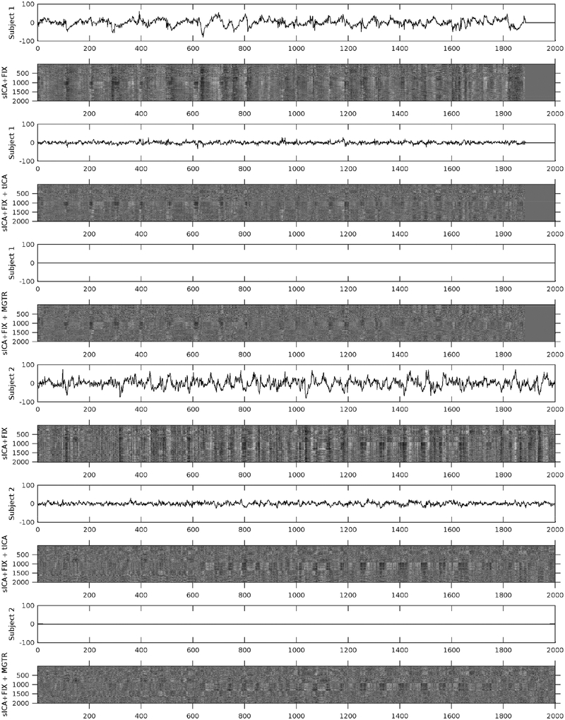
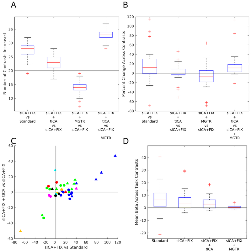
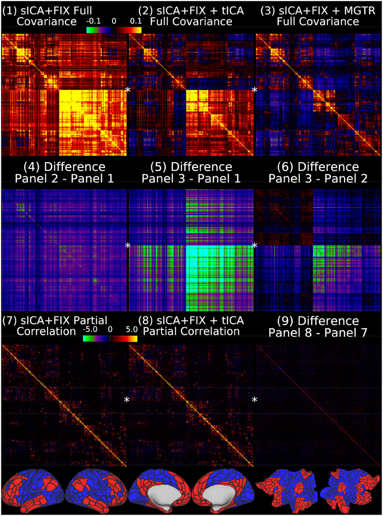
Temporal fluctuations in functional Magnetic Resonance Imaging (fMRI) have been profitably used to study brain activity and connectivity for over two decades. Unfortunately, fMRI data also contain structured temporal "noise" from a variety of sources, including subject motion, subject physiology, and the MRI equipment. Recently, methods have been developed to automatically and selectively remove spatially specific structured noise from fMRI data using spatial Independent Components Analysis (ICA) and machine learning classifiers. Spatial ICA is particularly effective at removing spatially specific structured noise from high temporal and spatial resolution fMRI data of the type acquired by the Human Connectome Project and similar studies. However, spatial ICA is mathematically, by design, unable to separate spatially widespread "global" structured noise from fMRI data (e.g., blood flow modulations from subject respiration). No methods currently exist to selectively and completely remove global structured noise while retaining the global signal from neural activity. This has left the field in a quandary-to do or not to do global signal regression-given that both choices have substantial downsides. Here we show that temporal ICA can selectively segregate and remove global structured noise while retaining global neural signal in both task-based and resting state fMRI data. We compare the results before and after temporal ICA cleanup to those from global signal regression and show that temporal ICA cleanup removes the global positive biases caused by global physiological noise without inducing the network-specific negative biases of global signal regression. We believe that temporal ICA cleanup provides a "best of both worlds" solution to the global signal and global noise dilemma and that temporal ICA itself unlocks interesting neurobiological insights from fMRI data.


Figures

Figure 1
Figure 1
shows an overview of the methods of the paper from the preprocessed dense timeseries to the final analysis outputs. Data are blue and algorithms are green. Data or algorithms with a thicker outline were run on a per-subject or per run basis. All 449 subjects of both resting state and task data were run through the process; however, only the 210P subgroup was used in the group dense functional connectivity and gradient analysis for computational reasons (210P and 210V groups of subjects have a correlation of r=0.98 in their group functional connectivity, (Glasser et al., 2016a)).
Figure 2
Figure 2
shows the first task fMRI tICA component in a standardized display format (see also Supplementary Figures TC 1–70). The top row of data has the color scale normalized and held constant across all 70 components (in percent BOLD), whereas the second row has the color scale set independently for each component. Hence the first view allows components to be compared with each other on the same scale, whereas the second view highlights patterns in the map of each specific component and is scaled between 0% and 98%. The left chart in the third row indicates the power spectrum of the component averaged across subjects, and the right chart indicates the average timeseries (red) and average absolute value of the timeseries (green). Both of these will show evidence of the task stimulus for task-modulated components because of consistent task timing across subjects. Additional information about the component is provided in the table along the bottom row (see Figures 3 and 4 for thresholds that determine Yes/No status, which is also sortable in the Supplementary Component Data Table). The rationale for classifying the component is listed along the bottom row of the table. Supplementary Figure 4 shows how the task fMRI runs were concatenated. Percent variance explained is computed using the ‘total variance’ of the data at the tICA modeling stage (i.e., after sICA+FIX cleaning and the d=137 sICA dimensionality reduction, and thus sums to 100% across all the tICA signal and noise components). The globality index is abs(ln2(# positive grayordinates/# negative grayordinates)). Data at https://balsa.wustl.edu/m9k0.
Figure 3
Figure 3
shows four plots that were helpful during task fMRI component classification into signal and noise. Panel A is the correlation between the component timeseries and RVT for the 70 concatenated task sessions that had the top 10% mean correlation between RVT and their parcellated fMRI data. This selects for subjects having both good quality RVT traces and substantial respiratory contamination of their data (see Methods Section #1.6). The line is at r=0.1. Panel B is the difference in component amplitude (standard deviation of the component timeseries) between frames with DVARS dips and those without DVARS dips normalized by the component amplitude across all frames (see Methods Section #1.9), so as to highlight those components that have stronger temporal fluctuations during DVARS dips. The line is at 0.18. Panel C shows the variability of component amplitudes across subjects normalized by the overall amplitude of each component. The line is at 0.15. Panel D shows the difference between the maximum subject’s component amplitude and the next highest subject’s component amplitude normalized by the overall amplitude of each component. This measure highlights those components that are particularly strong in a single subject. The line is at 0.4. The discriminatory thresholds in this figure and in Figure 7 and Supplementary Figure 16 were chosen as described in Methods Section #1.9. Those components above each threshold are numbered on each graph.
Figure 4
Figure 4
shows the component amplitudes modulated by task. The measure is the amplitude of a component (standard deviation over time) during a given task versus all other tasks (std(SpecificTask)-std(AllOtherTasks)). Task abbreviations are WM=Working Memory, GMB=Gambling, MOT=Motor, LAN=Language, SOC=Social, REL=Relational, and EMO=Emotion. The top panel shows the original task component amplitudes (70) whereas the bottom panel shows the component amplitudes after regressing out the task GLM (58 reproducible components). The line is at 0.25 in both cases.
Figure 5
Figure 5
shows the mean grey signals and parcellated greyplots of two concatenated task fMRI timeseries from two subjects after sICA+FIX (Rows 1–2, 7–8), sICA+FIX + tICA (Rows 3–4, 9–10), and sICA+FIX + MGTR (Rows 5–6, 11–12). Note that concatenated session 1 is shorter than concatenated session 2 and so the first 3 rows include zero-padding on the far right. The data were parcellated as described in the methods, then displayed according to parcel surface area (with 1 row assigned for the smallest parcel and proportionally larger numbers of rows assigned for larger parcels such that there are more than 360 rows). Additionally, the data are ordered by hierarchical clustering of the group full correlation parcellated connectome so that parcels with more similar timeseries across the group are closer together (see the bottom row of Figure 13 which shows the “cognitive/task negative vs non-cognitive/task positive split that forms the primary clustering split about half way down the y-axis in the grey plots). tICA cleanup removes the vertical “stripes” (signal deviations of the same sign across the whole brain) from the greyplots that were present after sICA+FIX and their corresponding MGT fluctuations, but without removing the entire MGT as occurs with MGTR. The greyplots after tICA cleanup and MGTR look similar but not identical. The greyscale ranges from −2% to +2% BOLD.
Figure 6
Figure 6
compares the statistical sensitivity (Panels A, B, and C) and mean beta values (Panel D) across contrasts and cleanup approaches. Statistical sensitivity was quantified via the cluster mass using a Z=+/− 5 threshold. Panel A shows the number of contrasts found to have increased cluster mass using a box and whisker plot for sICA+FIX vs Standard, sICA+FIX + tICA vs sICA+FIX, and sICA+FIX + MGTR vs sICA+FIX, and sICA+FIX + tICA vs sICA+FIX + MGTR for 100 random subsets of 28 subjects from the 449 total subjects. Only primary contrasts that are not averages of other primary contrasts and differential contrasts are plotted with no negative duplicates (n=40 contrasts out of the total of 86 released by the HCP). The Gambling REWARD-PUNISH contrast has minimal neural signal (Glasser et al., 2016a) and thus acts as a negative control (golden triangle in (C)). The red line is the median, the edges of the box are the 25th and 75th percentiles, the whiskers are at the data point closest to +/− 2.7 standard deviations (the robust range), and the outliers (+’s) are the data points beyond these thresholds. The horizontal black line is at 20 (of 40 total) contrasts improving (50%). Panel B shows the percent change in cluster mass for the tfMRI contrasts for the same comparisons, with a horizontal black line at 0% change (the percent change for each contrast is the average across 100 random subsets and the boxplot shows the distribution across contrasts). Panel C shows a scatter plot of the percent improvement of cluster mass from sICA+FIX over standard processing vs the improvement of sICA+FIX + tICA over sICA+FIX processing. Circles are primary contrasts and triangles are differential contrasts. The colors are the same as used in Figure 4 to represent the different tasks. Panel D shows the spatial means across the entire contrast beta maps for standard processing, sICA+FIX, sICA+FIX + tICA, and sICA+FIX + MGTR.
Figure 7
Figure 7
shows four plots that were helpful in classifying the resting state fMRI tICA components into signal and noise. Panel A shows the correlation between the component timeseries and RVT for the 157 runs with the top 10% mean correlation between RVT and their parcellated timeseries as in Figure 3. When the 3 global components timeseries (RC3, 6, and 8) are added together, the correlation with RVT is 0.28, very similar to the correlation of the single task global component (0.30) with RVT. The line is at r=0.1. Panel B is the difference in component amplitude (standard deviation of the component timeseries) between frames with DVARS dips and those without DVARS dips normalized by the standard deviation of each component across all frames as in Figure 3. The line is at 0.1. Panel C shows the variability of component amplitudes across subjects normalized by the standard deviation of each component as in Figure 3. The line is at 0.2. Panel D shows the difference between the maximum subject’s component amplitude and the next highest subject’s component amplitude normalized by the standard deviation of each component as in Figure 3. The line is at 1.0.
Figure 8
Figure 8
shows the first resting state fMRI tICA component in a standardized display format (see Supplementary Figures RC 1–84). The top row of data has the color scale normalized and held constant across all 84 components (in percent BOLD), whereas the second row has the color scale set independently for each component (scaled between 2nd and 98th percentiles for that component). The first view allows components to be compared with each other on the same scale, whereas the second view highlights spatial variation in the map of each specific component. The left chart in the third row indicates the power spectra of the component averaged across subjects and the right chart indicates the average timeseries (red) and average absolute value of the timeseries (green). The increasing trend of the absolute average timeseries across the run (which is like an average instantaneous component amplitude) is likely indicative of subjects progressively becoming drowsy or falling asleep. The timeseries are concatenated in the order that the runs were typically acquired (REST1_RL, REST1_LR, REST2_LR, REST2_RL) to enable visualization of trends across the two sessions. Additional data on the components is provided in the table along the bottom row. The classification rationale appears along the bottom row of the table. Percent variance explained and the globality index are computed as explained in Figure 2. Data at https://balsa.wustl.edu/kLpN.
Figure 9
Figure 9
shows two useful sleep related component measures. The top row is the difference in component amplitude in subjects that were noted to be sleeping vs those who were not. The bottom row shows the difference in component amplitude between the last 300 frames and the first 300 frames of the 1200 frame runs, as subjects will presumably be more likely to be asleep at the end of a 14.4 minute run than at the beginning. Components 47, 58, and 80 are “single subject” components that are unlikely to be specifically sleep related. The 3 global physiological noise components (RC3, 6, and 8) are all also more likely to be higher at the end of a run than at the beginning, likely indicating greater respiratory variability at the end of runs when subjects are more likely to be drowsy. This is also true of noise component 25. Otherwise, these two measures agree on the components most likely to be related to sleep.
Figure 10
Figure 10
shows the mean grey signals and parcellated greyplots for two resting state fMRI runs from two subjects after sICA+FIX (Rows 1–2, 7–8), sICA+FIX + tICA (Rows 3–4, 9–10), and sICA+FIX + MGTR (Rows 5–6, 11–12). The data are parcellated, then displayed according to parcel surface area (with 1 row assigned for the smallest parcel and proportionally larger numbers of rows assigned for larger parcels such that there are more than 360 rows). Additionally, the data are ordered by hierarchical clustering of the group full correlation functional connectome after sICA+FIX + tICA so that parcels with more similar timeseries are closer together. tICA cleanup removes the vertical “stripes” from the grey plots after sICA+FIX and their corresponding MGT fluctuations without removing the entire MGT as occurs with MGTR. The greyplots after tICA cleanup and MGTR look very similar, although the tICA cleanup plots retain more semi-global structure.
Figure 11
Figure 11
shows the results of group grayordinate-wise functional connectivity and functional connectivity gradient maps after sICA+FIX, sICA+FIX + tICA, and sICA+FIX + MGTR for the 210P subject group. The top row shows a seed in left hemisphere area V1 (circled) that has generally positive correlation with other grayordinates after sICA+FIX, positive to zero correlation after sICA+FIX + tICA, and widespread negative correlation induced by sICA+FIX + MGTR. The second row shows a seed in left hemisphere Area PGi (circled), which shows much more similar maps in an already anti-correlated network that is not as affected by MGTR. The third row shows the mean gradients after each kind of processing, with the gradients after sICA+FIX and sICA+FIX + tICA matching well (with an increase in gradient strength after tICA cleanup), whereas the gradients after MGTR shift in several regions highlighted by the outlined cortical areas (in white). The fourth row zooms in on several regions showing gradient shift after MGTR. Data at https://balsa.wustl.edu/6mV1.
Figure 12
Figure 12
shows the entire full correlation parcellated connectome computed by parcellating the MIGP PCA series that was the input to the analyses in Figure 11 to show an overall summary of the trends in this data. It has sICA+FIX + tICA (x-axis) plotted vs sICA+FIX (y-axis; blue) on the left, showing a positive bias in sICA+FIX, and sICA+FIX + tICA plotted vs sICA+FIX + MGTR (red) in the middle, showing a negative bias in sICA+FIX + MGTR. Histograms of the correlation values are shown on the right with sICA+FIX blue, sICA+FIX + tICA green, and sICA+FIX + MGTR red, illustrating that sICA+FIX + tICA falls roughly halfway between sICA+FIX and sICA+FIX + MGTR.
Figure 13
Figure 13
shows the group average full covariance matrices after sICA+FIX, sICA+FIX + tICA, and sICA+FIX + MGTR in Panels 1–3. We use covariance here because, like variances, covariances are additive and represent the absolute amount of variance shared by any two pairs of ROIs (scaled from −0.1 to 0.1 in percent BOLD for Panels 1–6). As in other figures, a global positive bias is removed by tICA cleanup (Panel 4 shows the difference between Panel 2 and Panel 1), but MGTR also removes additional signal in the bottom right quadrant of the matrix relative to the upper left quadrant with the off-diagonal quadrants in between (Panel 5 shows the difference between Panel 3 and Panel 1). Importantly, the difference between the tICA cleanup and MGTR (Panel 6 shows the difference between Panel 3 and Panel 2) is highly network specific, including small increases in cognitive/task-negative regions (bottom row, parcels shown in red) and large decreases in primarily non-cognitive/task positive regions (bottom row, blue parcels), with connections between the parcels of these two broad groups of regions showing smaller decreases. Panels 7 and 8 show that mean across subjects partial correlation regularized with ridge regression (rho=0.23, which was optimal in matching the individual matrices to the group matrix computed with no regularization; scaled Z=+/−5) is much less affected by tICA cleanup, as it already controls for global artifacts (Glasser et al., 2016b). Thus, Panel 9 (difference between Panel 8 and Panel 7) does not reveal substantial differences. The 360 cortical areas are ordered according to the same hierarchical clustering as the grey plots, and the first split, into cognitive/task negative (red) and non-cognitive and task positive (blue) regions, is shown in the bottom row and noted by a star on the netmats, with red parcels in the upper left quadrant of the netmats, and the blue parcels in the lower right quadrant. Note that it would be inappropriate to use partial correlation after MGTR, as any dataset that has zero global signal is rank deficient, because each parcel’s timeseries equals the negated sum of all other parcels’ timeseries. Data at https://balsa.wustl.edu/1lBX.

Comment in

References

    1. Aguirre GK, Zarahn E, and D’Esposito M. 1997. Empirical analyses of BOLD fMRI statistics. II. Spatially smoothed data collected under null-hypothesis and experimental conditions. NeuroImage. 5:199–212. - PubMed
    1. Aguirre GK, Zarahn E, and D’Esposito M. 1998. The inferential impact of global signal covariates in functional neuroimaging analyses. NeuroImage. 8:302–306. - PubMed
    1. Anderson JS, Druzgal TJ, Lopez-Larson M, Jeong EK, Desai K, and Yurgelun-Todd D.2011. Network anticorrelations, global regression, and phase-shifted soft tissue correction. Human brain mapping. 32:919–934. - PMC - PubMed
    1. Barch DM, Burgess GC, Harms MP, Petersen SE, Schlaggar BL, Corbetta M, Glasser MF, Curtiss S, Dixit S, Feldt C, Nolan D, Bryant E, Hartley T, Footer O, Bjork JM, Poldrack R, Smith S, Johansen-Berg H, Snyder AZ, and Van Essen DC. 2013. Function in the human connectome: task-fMRI and individual differences in behavior. NeuroImage. 80:169–189. - PMC - PubMed
    1. Behzadi Y, Restom K, Liau J, and Liu TT. 2007. A component based noise correction method (CompCor) for BOLD and perfusion based fMRI. NeuroImage. 37:90–101. - PMC - PubMed

Publication types