Sharpening of Hierarchical Visual Feature Representations of Blurred Images

Abstract

The robustness of the visual system lies in its ability to perceive degraded images. This is achieved through interacting bottom-up, recurrent, and top-down pathways that process the visual input in concordance with stored prior information. The interaction mechanism by which they integrate visual input and prior information is still enigmatic. We present a new approach using deep neural network (DNN) representation to reveal the effects of such integration on degraded visual inputs. We transformed measured human brain activity resulting from viewing blurred images to the hierarchical representation space derived from a feedforward DNN. Transformed representations were found to veer toward the original nonblurred image and away from the blurred stimulus image. This indicated deblurring or sharpening in the neural representation, and possibly in our perception. We anticipate these results will help unravel the interplay mechanism between bottom-up, recurrent, and top-down pathways, leading to more comprehensive models of vision.

Keywords: Decoding; Deep Neural Network; fMRI.

Graphical abstract

Figure 1.

Study design. A, The stimulus sequence was divided into sequences of four stimuli each. Stimuli in the same sequence contained different blur levels of the same image organized from the highest blur level (25%) to the lowest (0%). Each stimulus was presented for 8 s. B, Overview of the feature decoding analysis protocol; fMRI activity was measured as the subjects viewed the stimulus images presented, described in A. Trained decoders were used to predict DNN features from fMRI activity patterns. The decoded features were then analyzed for their similarity with the true DNN features of both the original image (r_o) and stimulus image (r_s). The same procedure was also conducted for noise-matched DNN features that are composed of true DNN features with additional Gaussian noise to match predicted features from fMRI.

Figure 2.

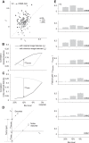
Correlation of decoded features with original and stimulus image features. A, Scatter plot showing feature correlation of DNN6 features decoded from the whole visual cortex (VC) of subject 4, with stimulus image features (r_s; x-axis) and original image features (r_o; y-axis). Each point represents a stimulus image for all blurring levels except 0%, while the white points with black borders show the mean of all points of the same blur level. Diagonal dotted line represents the line of equal correlation (Δr_decode = 0). B, Representative result from DNN6 features decoded from the whole VC of subject 4. Lines represent the mean correlation at different blur levels while pooling different experimental conditions and behavioral response data. The difference between r_o and r_s is labeled as Δr_decode. C, Representative result showing mean noise-matched feature correlation with the original and stimulus image features for different blur levels. Noise-matching was performed to match the correlation of the DNN6 predicted features of the 0% blur stimuli decoded from VC of subject 4 (thus obtaining equal values with the decoded features at the 0% level). The difference between r_o and r_s yields the noise baseline (Δr_noise). D, Feature gain is defined as the difference between Δr_decode and Δr_noise. Δr could be defined as the displacement along the r_o axis of the point on the plot from the line of equal correlation. So by subtracting the vector representing noise-matched feature correlations from decoded feature correlation, we can calculate feature gain. E, Mean feature gain is indicated for each DNN layer for features decoded from VC at different stimulus blur levels (excluding the 0% level). Error bars indicate 95% confidence interval (CI) across five subjects.

Figure 3.

Content specificity of decoded features with blurred images. Same image correlation indicates correlation of predicted features (blur levels pooled, excluding 0%) with corresponding original image features. Different images correlation indicates the mean of correlations of the same predicted features with original image features of different images. The mean correlation is shown for different DNN layers. Error bars indicate 95% CI across five subjects.

Figure 4.

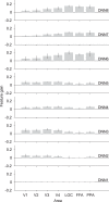
Feature gain across visual areas. Feature gain for features predicted from different visual areas. Mean feature gain is indicated for each DNN layer (blur levels pooled, 0% excluded). Error bars indicate 95% CI across five subjects.

Figure 5.

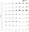
Effect of category prior. Feature gain for features predicted from different visual areas grouped by experimental condition (category-prior vs. no-prior). Mean feature gain is indicated for each DNN layer (blur levels pooled, 0% excluded). Error bars indicate 95% CI across five subjects.

Figure 6.

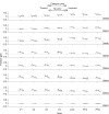
Effect of behavioral performance. Feature gain for features predicted from different visual areas grouped by experimental condition (category-prior vs. no-prior) and recognition (correct vs. incorrect). Legends include the total number of occurrences of each response across subjects. Mean feature gain is indicated for each DNN layer (blur levels pooled, 0% excluded). Error bars indicate 95% CI across five subjects.

Figure 7.

Effect of confidence level. Feature gain for features predicted from different visual areas grouped by experimental condition (category-prior vs. no-prior) and confidence level (certain vs. uncertain). Legends include the total number of occurrences of each response across subjects. Mean feature gain is indicated for each DNN layer (blur levels pooled, 0% excluded). Error bars indicate 95% CI across five subjects.

References

1. Ahissar M, Hochstein S (2004) The reverse hierarchy theory of visual perceptual learning. Trends Cogn Sci (Regul Ed) 8:457–464. 10.1016/j.tics.2004.08.011 - DOI - PubMed
1. Alink A, Schwiedrzik CM, Kohler A, Singer W, Muckli L (2010) Stimulus predictability reduces responses in primary visual cortex. J Neurosci 30:2960–2966. 10.1523/JNEUROSCI.3730-10.2010 - DOI - PMC - PubMed
1. Arnal LH, Giraud A-L (2012) Cortical oscillations and sensory predictions. Trends Cogn Sci (Regul Ed) 16:390–398. 10.1016/j.tics.2012.05.003 - DOI - PubMed
1. Bansal A, Sheikh Y, Ramanan D (2017) PixelNN: Example-based image synthesis. arXiv Preprint arXiv 170805349.
1. Bar M, Aminoff E (2003) Cortical analysis of visual context. Neuron 38:347–358. - PubMed
Publication types
LinkOut - more resources