Two-photon imaging of neuronal activity in motor cortex of marmosets during upper-limb movement tasks

Abstract

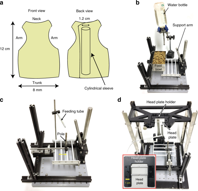
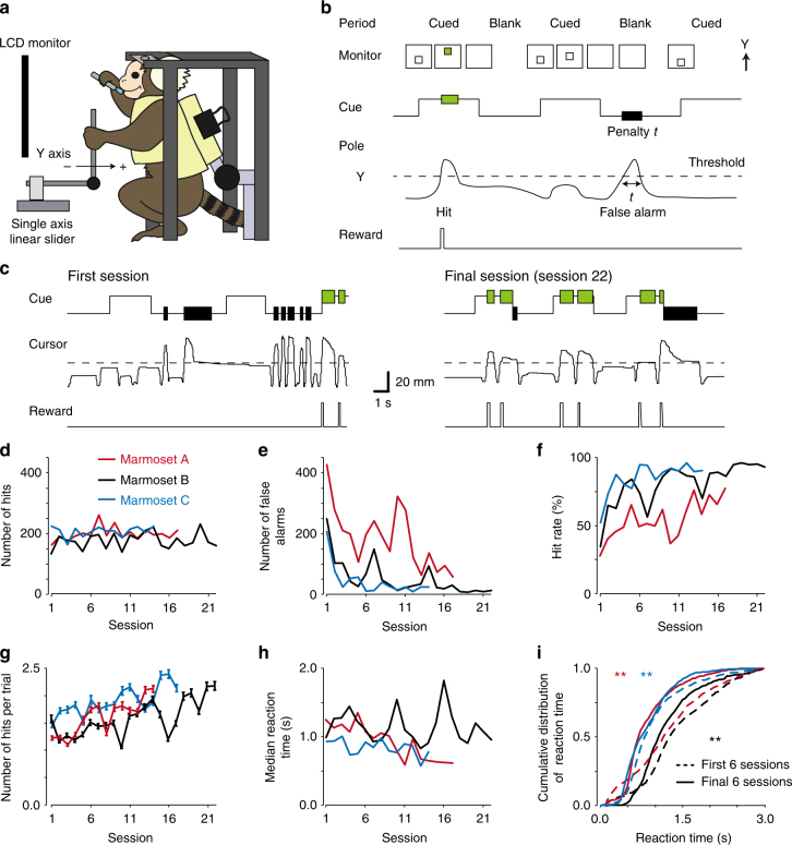
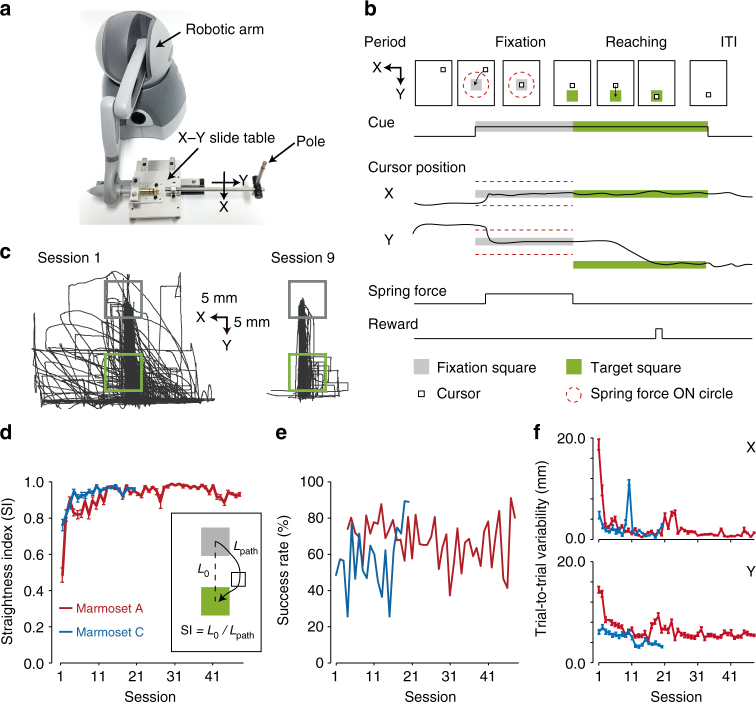
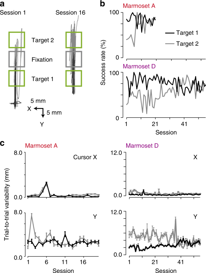
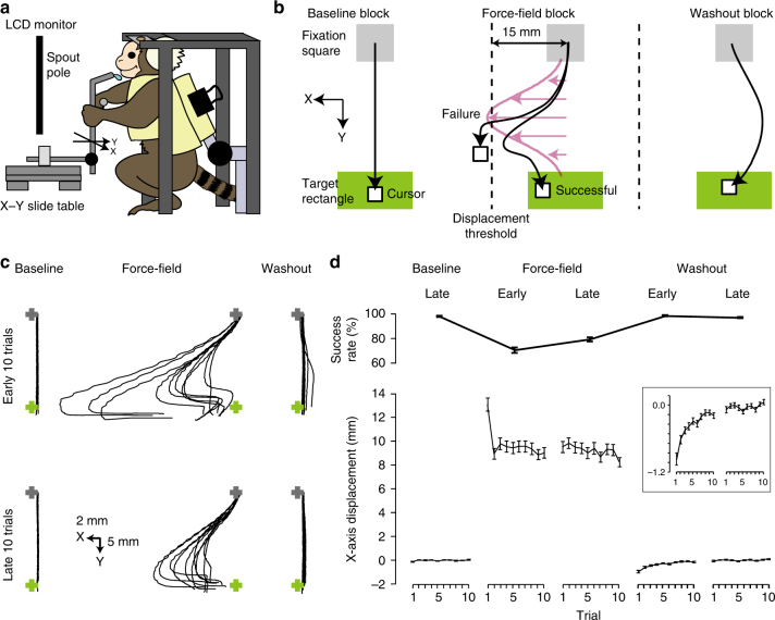
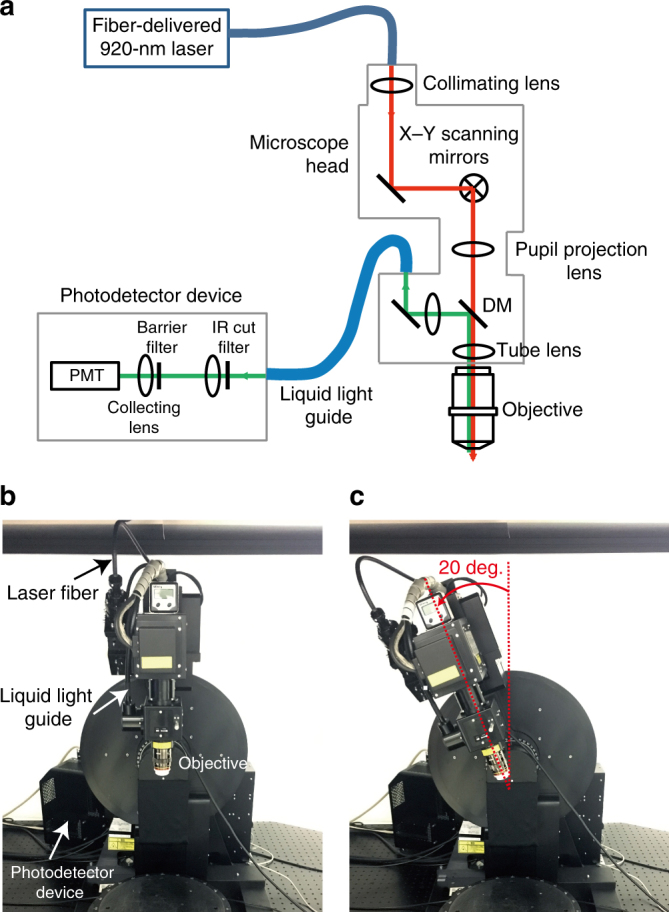
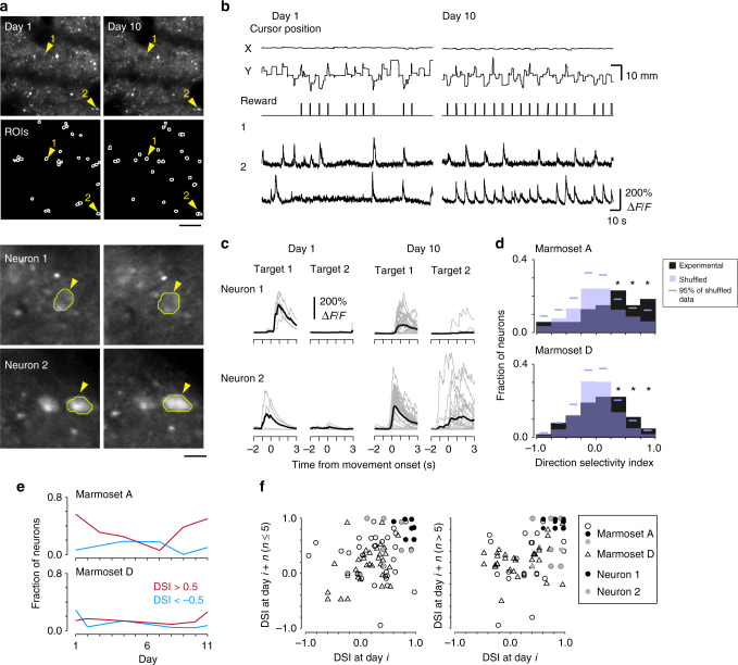
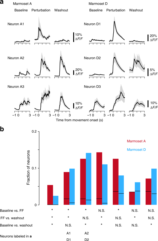
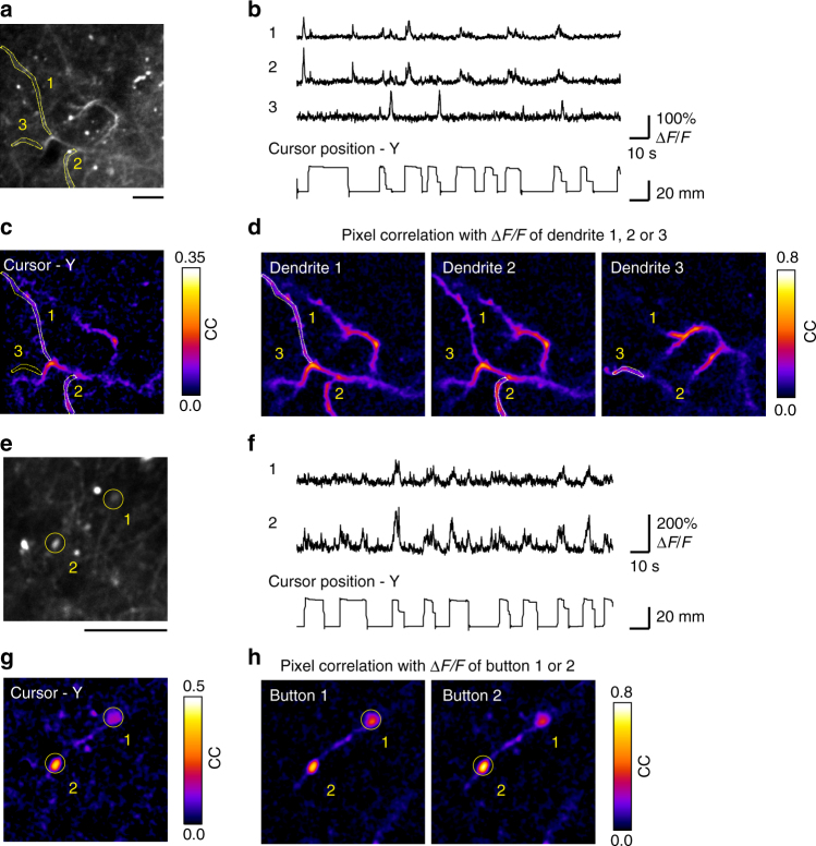
Two-photon imaging in behaving animals has revealed neuronal activities related to behavioral and cognitive function at single-cell resolution. However, marmosets have posed a challenge due to limited success in training on motor tasks. Here we report the development of protocols to train head-fixed common marmosets to perform upper-limb movement tasks and simultaneously perform two-photon imaging. After 2-5 months of training sessions, head-fixed marmosets can control a manipulandum to move a cursor to a target on a screen. We conduct two-photon calcium imaging of layer 2/3 neurons in the motor cortex during this motor task performance, and detect task-relevant activity from multiple neurons at cellular and subcellular resolutions. In a two-target reaching task, some neurons show direction-selective activity over the training days. In a short-term force-field adaptation task, some neurons change their activity when the force field is on. Two-photon calcium imaging in behaving marmosets may become a fundamental technique for determining the spatial organization of the cortical dynamics underlying action and cognition.

Fig. 1

Design of the task apparatus. a Layout of the jacket modified from Schultz-Darken et al. . The jacket has openings for the neck, arms, and trunk to pass through. The girth of the trunk was adjusted with a hook-and-loop fastener. The illustrations of the back view show the cylindrical sleeve used to restrain the trunk. b Apparatus for habituation to trunk constraint. The support arm was inserted through the cylindrical sleeve and restrained the trunk of the marmoset. The support arm and the cylindrical sleeve were fixed by a clip. The marmoset grasped the white scaffolding with leg paws, ate food pellets from the food bowl with upper limbs, and drank drops from the water bottle. c Apparatus for the self-initiated pole-pull task. The yellow double-headed arrow indicates the range in which the pole could move (3.5 cm). d A head plate was clamped by a head plate holder (inset), and the head plate holder was clamped by the apparatus

Fig. 2

Learning of visually cued pole-pull task. a Scheme of the task apparatus and head-fixed marmoset. b Schematic diagram of the task. c Example of pole trajectories from marmoset B. d–g Time course of the hit number (d), the false alarm number (e), the hit rate (f), and the hit number per trial (g) across sessions. In g, only trials with at least one hit event were analyzed (n = 73–183 trials for each session). Error bars indicate SEM. Spearman correlation coefficients (CCs) between the hit number and training session were 0.35, 0.09, and 0.07 (0.22, −0.04, and 0.33 without the initial session) for marmosets A, B, and C, respectively, P > 0.05 for all cases. CCs between the false alarm number and training session were −0.72, −0.79, and −0.58 for marmosets A, B, and C, respectively, P < 0.01 for marmosets A and B, P < 0.05 for marmoset C. Without the initial session, CCs were –0.66, –0.76, and –0.47 for marmosets A, B, and C, respectively, P < 0.01 for marmosets A and B, P = 0.10 for marmoset C. CCs between the hit rate and training session were 0.72, 0.84, and 0.67 (0.66, 0.82, and 0.59 without the initial session) for marmosets A, B, and C, respectively, P < 0.01 for marmosets A and B, P < 0.05 for marmoset C. CCs between the hit number per trial and training session were 0.81, 0.71, and 0.81 (0.77, 0.77, and 0.77 without the initial session) for marmosets A, B, and C, respectively; P < 0.01. h Median reaction time. i The cumulative distribution of reaction time. For marmoset A: 1203 ± 29 ms in the first six sessions vs. 833 ± 21 ms in the final six sessions, n = 664 and 578 trials, respectively, **P < 0.01, Wilcoxon rank-sum test. For marmoset B: 1396 ± 26 ms vs. 1207 ± 25 ms, n = 763 and 569 trials, respectively, **P < 0.01. For marmoset C: 1032 ± 18 ms vs. 904 ± 17 ms, n = 952 and 673 trials, respectively, **P < 0.01

Fig. 3

Learning of the one-target reaching task. a An X–Y slide table to enable marmosets to control the pole on a 2D working space (53 mm for the X-axis and 90 mm for the Y-axis). A robotic arm was connected to the table. b The task consisted of fixation and reaching periods, and an inter-trial interval (ITI). During the reaching period, a target (green) was presented and marmosets used the manipulandum to move the cursor from a fixation square (gray) to the target and hold it for 10–300 ms to obtain a reward. c Reaching trajectories in sessions 1 and 9 in marmoset A. Each trajectory for each trial is overlaid. Gray and green boxes indicate the fixation and target squares, respectively. d Time course of the mean straightness index (SI) of the successful reaching trajectory in marmosets A (red) and C (blue). CCs between SI and the training session were 0.48 (0.45 without the initial session) for marmoset A (P < 0.01) and 0.70 (0.65 without the initial session) for marmoset C (P < 0.01). e Time course of the success rate. The success rate was calculated by dividing the number of rewarded trials by that of all trials. The success rate in marmoset C was relatively low until session 15, because marmoset C had difficulties in stopping and holding the cursor within the target square, and the cursor frequently passed through it, even though the trajectory became straighter. f Time course of the trial-to-trial variability (see Methods) of X (top) and Y (bottom) coordinates for the successful reaching trajectories in marmosets A (red) and C (blue). The CCs between mean of the root mean square deviations (RMSDs) of X and Y coordinates and the session number in marmoset A were −0.58 (–0.55 without the initial session) and −0.55 (–0.52 without the initial session), respectively, P < 0.01, while for marmoset C they were −0.44, P = 0.054 (–0.36 without the initial session, P = 0.12), for the X coordinate, and −0.85 (–0.83 without the initial session), P < 0.01, for the Y coordinate

Fig. 4

Learning of the two-target reaching task. a Reaching trajectories in sessions 1 and 16 of the two-target reaching task in marmoset A. Black and gray solid lines represent reaching trajectories for the targets below (target 1) and above (target 2) the fixation square, respectively. Other conventions are the same as in Fig. 3c. b Time course of the success rates for different targets in marmosets A (top) and D (bottom). CCs between the success rate for target 1 and session number were −0.23 for marmoset A, P = 0.32, and −0.44 for marmoset D, P < 0.01. CCs between the success rate for target 2 and session number were 0.68 for marmoset A, P < 0.01, and 0.61 for marmoset D, P < 0.01. c Time course of the trial-to-trial variability of the successful reaching trajectory to targets 1 (black) and 2 (gray) in marmosets A (left) and D (right). For marmoset A, CCs between the variability of the reaching target 1 and session number were −0.05 and 0.01, P = 0.84 and P = 0.97, for X and Y coordinates, respectively. CCs for the variability of reaching target 2 were 0.25 and −0.18, P = 0.27 and P = 0.44, for X and Y coordinates, respectively. For marmoset D, CCs for the variability of reaching target 1 were 0.08 and 0.72, P = 0.54 and P < 0.01, for X and Y coordinates, respectively. CCs for the variability of reaching target 2 were −0.39 and −0.64, P < 0.01 and P < 0.01, for X and Y coordinates, respectively. Marmoset D demonstrated a slow learning rate for reaching target 2, with the variability for reaching target 1 increasing. This might be because marmoset D had performed the one-reaching task with a force field for approximately 30 days, and had become heavily habituated to reaching target 1

Fig. 5

Learning of the force-field adaptation task. a Scheme of the task apparatus. In this task, the handling pole was replaced with the spout pole and the marmoset manipulated it to move the cursor on the monitor. A fixed pole was put in front of the marmoset’s right arm to keep the right arm relaxed. b The target rectangle was placed below the fixation square. The width of the target rectangle was twice its height. During the FF block, a velocity- (in Y-axis direction) dependent force field was applied to the pole in the X-axis direction (representing the left direction in the hand workspace). c Example of the reaching trajectories in the first baseline, first force-field, and first washout blocks in session 2 from marmoset A. Gray and green crosses indicate the centers of the fixation square and target rectangle, respectively. d Success rate averaged over ten trials (top) and X-axis displacement of each trial (bottom) in consecutive baseline, force-field, and washout blocks (n = 117 from three marmosets). The early and late trials were the first ten and final ten reaching trials in each block. Success rate was the percentage of successful trials out of the ten trials. In the inset, the X-axis displacement in the washout block is magnified. Error bars indicate SEM

Fig. 6

Overview of the two-photon microscope for head-fixed marmosets. a Scheme of the optical pathway. The laser beam was directly introduced to the microscope head with x–y scanners. Thus, the wavefront of the laser at the exit of the objective was not affected by the tilt of the microscope body. The scanners consisted of a resonant mirror and a Galvano mirror. Emitted fluorescence was spilt by a dichromic mirror (DM; reflection and transmission wavelength ranges, 400–755 nm and 800–1300 nm, respectively), introduced to a liquid light guide, filtered by an IR cutting filter (wavelength range, 400–760 nm; 32BA750 RIF, Olympus) and a barrier filter (FV30-FGR), and then collected by a cooled high-sensitivity photomultiplier tube (PMT). b Non-tilt body position of the microscope body. c Body position with a tilt angle of 20° around the front-to-back axis

Fig. 7

In vivo two-photon multi-day imaging in the motor cortex during the reaching task. a Time-averaged two-photon images of GCaMP6f from marmoset A on imaging days 1 and 10 (first row), and ROIs identified by the CNMF algorithm (second row). Magnified areas around neurons 1 (third row) and 2 (fourth row), and their contours, are also shown. Scale bars: 100 μm for the whole images and 15 μm for the magnified images. b X and Y positions of the cursor, reward timing, and the traces of motion-corrected raw fluorescence signals in two representative neurons from imaging days 1 and 10 shown in a. c Traces of denoised ΔF/F signals of neurons 1 and 2 aligned to the cursor movement onset. Gray and black traces represent individual trials and the average, respectively. d Histogram of DSI of neurons pooled from six imaging sessions (black boxes). Purple boxes and lines indicate the distributions of shuffling-averaged DSI from the trial shuffled data, and the 95th percentile of 1000-time shuffling in individual bins, respectively. For both marmosets, fractions in the three bins with >0.25 DSI were above the 95th values (*P < 0.05). e Fractions of neurons with DSI >0.5 (red) and <−0.5 (cyan) in each session. CCs between the fraction of the neurons with DSI >0.5 and the imaging day, −0.09 and −0.03, P = 0.91 and P = 1.0, in marmosets A and D, respectively; neurons with DSI <−0.5, −0.14 and −0.54, P = 0.80 and P = 0.29, in marmosets A and D, respectively. f Similarity in the DSI of the same task-relevant neurons between different imaging days. Each point represents the DSIs of the same neuron on an imaging day and a following day ≤5 days apart (left) or >5 days apart (right). The CCs for the DSIs with session intervals ≤5 days were 0.23 and 0.45 (n = 50 and 31, P < 0.05 for both cases) for marmosets A and D, respectively, while those for an interval >5 days were 0.45 and 0.30 (n = 33 and 35, P < 0.01 and P < 0.05), respectively

Fig. 8

Changes in neuronal activity during the force-field adaptation task. a The task-relevant activity of six representative neurons (three from marmoset A and three from marmoset D). Denoised ΔF/F traces were aligned to the cursor movement onset. Lines and shaded areas represent mean ± SEM (n = 12–20 successful trials occurring during imaging for each block). Neurons A3 and D3 did not show significant differences in activity between the three blocks (Kruskal-Wallis test, P = 0.53 and 0.14, respectively). b Fractions of seven groups of neurons that showed significantly different activity between the three blocks (Kruskal-Wallis test, P < 0.05) with respect to the task-relevant neurons for each marmoset. According to the significance in the post-hoc test (P < 1−[1–0.05]^1/3), these neurons were classified into seven groups. Red, marmoset A. Cyan, marmoset D. Asterisk indicates a statistical difference between the pair of blocks shown on the left. N.S. indicates a non-statistical difference. The bottom indicates which groups of neurons (A1, A2, D1, and D2) in a were assigned to. Black line in each fraction box indicates the 95th percentile of the fraction obtained from trial shuffled data. Fractions, except for that in the second row from the right in marmoset A, were larger than the corresponding 95th percentiles

Fig. 9

Two-photon imaging of subcellular activity in layer 1 of the M1 during the task. a Representative time-averaged two-photon image of dendritic compartments at a depth of 51 μm from the cortical surface in the M1 of marmoset D. Scale bar, 30 μm. b Motion-corrected ΔF/F traces of three representative dendritic compartments indicated by the numbers in a. The Y-axis trajectory of the pole is shown at the bottom. c Map of correlation coefficients between the Y-axis cursor trajectory and the ΔF/F trace in each pixel. d Map of correlation coefficients in the ΔF/F traces with ROI 1 (left), ROI 2 (middle), and ROI 3 (right). e Representative time-averaged two-photon image of axonal buttons at a depth of 46 μm in the M1 of marmoset D. Scale bar, 20 μm. Other conventions are the same as in a. f Motion-corrected ΔF/F traces of two representative axonal buttons indicated by the numbers in e. g Map of correlation coefficients between the Y-axis cursor trajectory and the ΔF/F trace in each pixel. h Maps of correlation coefficients for the fluorescence changes for ROI 1 (left), and ROI 2 (right)

References

1. Huber D, et al. Multiple dynamic representations in the motor cortex during sensorimotor learning. Nature. 2012;484:473–478. doi: 10.1038/nature11039. - DOI - PMC - PubMed
1. Peters AJ, Chen SX, Komiyama T. Emergence of reproducible spatiotemporal activity during motor learning. Nature. 2014;510:263–267. doi: 10.1038/nature13235. - DOI - PubMed
1. Masamizu Y, et al. Two distinct layer-specific dynamics of cortical ensembles during learning of a motor task. Nat. Neurosci. 2014;17:987–994. doi: 10.1038/nn.3739. - DOI - PubMed
1. Chen TW, et al. Ultrasensitive fluorescent proteins for imaging neuronal activity. Nature. 2013;499:295–300. doi: 10.1038/nature12354. - DOI - PMC - PubMed
1. Margolis DJ, et al. Reorganization of cortical population activity imaged throughout long-term sensory deprivation. Nat. Neurosci. 2012;15:1539–1546. doi: 10.1038/nn.3240. - DOI - PubMed
Publication types