Uncovering the drivers of host-associated microbiota with joint species distribution modelling

Abstract

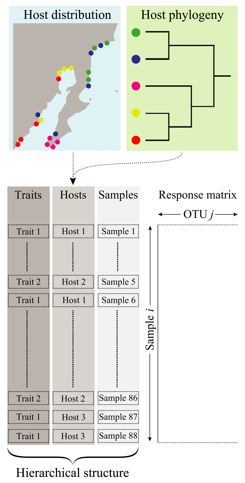
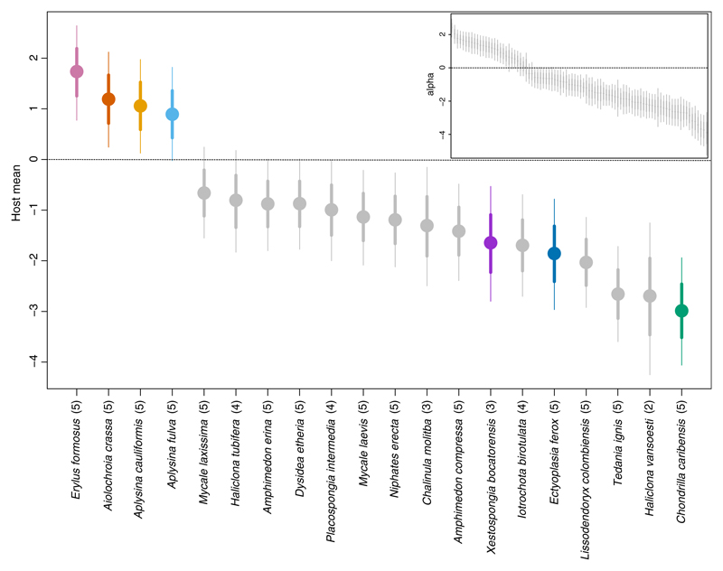
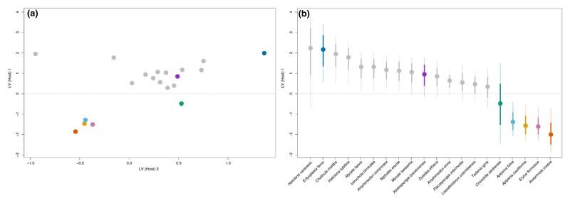
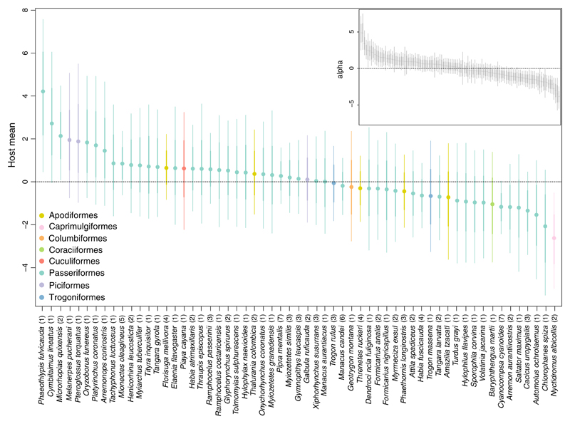
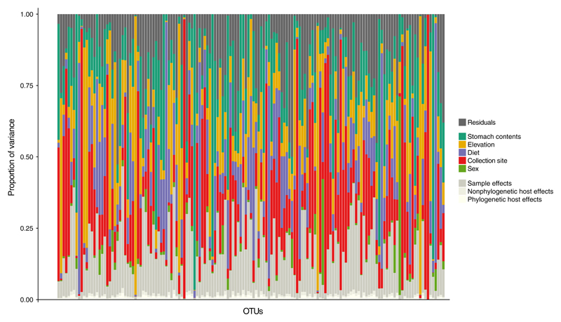
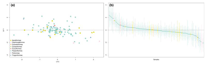
In addition to the processes structuring free-living communities, host-associated microbiota are directly or indirectly shaped by the host. Therefore, microbiota data have a hierarchical structure where samples are nested under one or several variables representing host-specific factors, often spanning multiple levels of biological organization. Current statistical methods do not accommodate this hierarchical data structure and therefore cannot explicitly account for the effect of the host in structuring the microbiota. We introduce a novel extension of joint species distribution models (JSDMs) which can straightforwardly accommodate and discern between effects such as host phylogeny and traits, recorded covariates such as diet and collection site, among other ecological processes. Our proposed methodology includes powerful yet familiar outputs seen in community ecology overall, including (a) model-based ordination to visualize and quantify the main patterns in the data; (b) variance partitioning to assess how influential the included host-specific factors are in structuring the microbiota; and (c) co-occurrence networks to visualize microbe-to-microbe associations.

Keywords: Bayesian inference; generalized linear mixed models; host-associated; joint species distribution models; microbiome; microbiota.

Figure 1

Host-associated microbiota data have a hierarchical data structure. In this example, samples are nested within host species which in turn are nested under species traits. Additional data often available are, e.g., (part of) the geographic distribution of the focal host species, as well as the phylogenetic relatedness between those. This means that host species can be further nested within observation/collection sites, and linked to branches in a phylogeny. The proposed model extension can straightforwardly accommodate for this hierarchical data structure and discriminate their importance in structuring the microbiota [Colour figure can be viewed at wileyonlinelibrary.com]

Figure 2

The main plot shows a caterpillar plot for the host means μ(host)_s, with the colours representing the seven HMA hosts. The subplot shows a caterpillar plot for the row effects α_i. The quantiles correspond to the 95% (thin lines) and 68% (thick lines) credible intervals, respectively. The number within the parentheses shows how many individuals per host species were availible to draw inference on [Colour figure can be viewed at wileyonlinelibrary.com]

Figure 3

Plot (a) shows the ordination constructed from the latent factors on the host species level Z^H, and plot (b) shows the corresponding caterpillar for first latent factor $Z_{i1}^H.$ The quantiles correspond to the 95% (thin lines) and 68% (thick lines) credible intervals, respectively [Colour figure can be viewed at wileyonlinelibrary.com]

Figure 4

The main plot shows a caterpillar for the host means μ(host)_s coloured by host taxonomy at the order level, while the subplot shows a caterpillar plot for the row effects α_i. The quantiles correspond to the 95% (thin lines) and 68% (thick lines) credible intervals, respectively. The number within the parentheses shows how many individuals per host species were availible to draw inference on [Colour figure can be viewed at wileyonlinelibrary.com]

Figure 5

The y-axis shows the relative proportion of variance in species occurrences explained by the hierarchy present on α_i, the covariates included on the linear predictor L_ij, and the residual variance not accounted for by the modelled effects, that is, the diagonal elements of the residual covariance matrix Ω, for each OTU (x-axis) [Colour figure can be viewed at wileyonlinelibrary.com]

Figure 6

Plot (a) shows the ordination constructed from the latent factors Z coloured by host taxonomy (at the order level) and plot (b) shows the corresponding caterpillar plot for the first latent factor Z_i1. The quantiles correspond to the 95% (thin lines) and 68% (thick lines) credible intervals, respectively [Colour figure can be viewed at wileyonlinelibrary.com]

References

1. Aivelo T, Norberg A. Parasite–microbiota interactions potentially affect intestinal communities in wild mammals. Journal of Animal Ecology. 2018;87(2):438–447. doi: 10.1111/1365-2656.12708. - DOI - PubMed
1. Balint M, Bahram M, Eren AM, Faust K, Fuhrman JA, Lindahl B, et al. Tedersoo L. Millions of reads, thousands of taxa: Microbial community structure and associations analyzed via marker genes. FEMS Microbiology Reviews. 2016;40(5):686. doi: 10.1093/femsre/fuw017. - DOI - PubMed
1. Berendsen RL, Pieterse CM, Bakker PA. The rhizosphere microbiome and plant health. Trends in Plant Science. 2012;17(8):478–486. doi: 10.1016/j.tplants.2012.04.001f. - DOI - PubMed
1. Bhattacharya A, Dunson DB. Sparse Bayesian infinite factor models. Biometrika. 2011;98:291–306. doi: 10.1093/biomet/asr013. - DOI - PMC - PubMed
1. Bolker BM, Brooks ME, Clark CJ, Geange SW, Poulsen JR, Stevens MHH, White JSS. Generalized linear mixed models: A practical guide for ecology and evolution. Trends in Ecology & Evolution. 2009;24(3):127–135. doi: 10.1016/j.tree.2008.10.008. - DOI - PubMed
Publication types
LinkOut - more resources