Iron-specific Signal Separation from within Heavy Metal Stained Biological Samples Using X-Ray Microtomography with Polychromatic Source and Energy-Integrating Detectors

Abstract

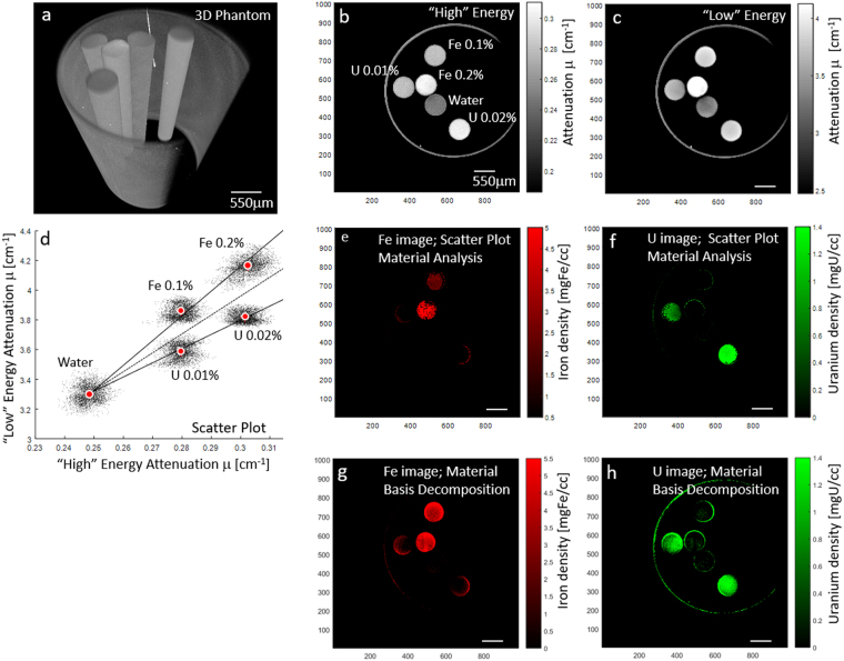
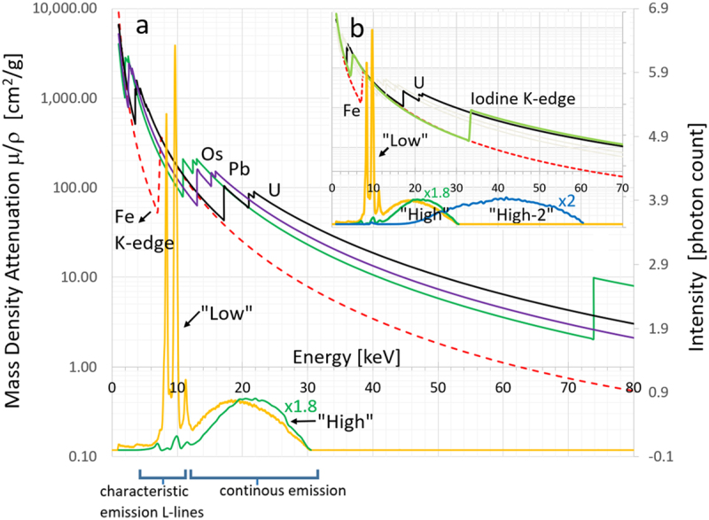
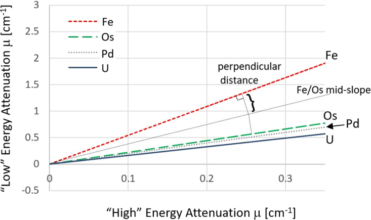
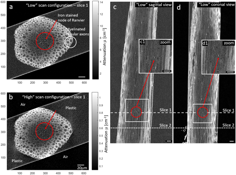
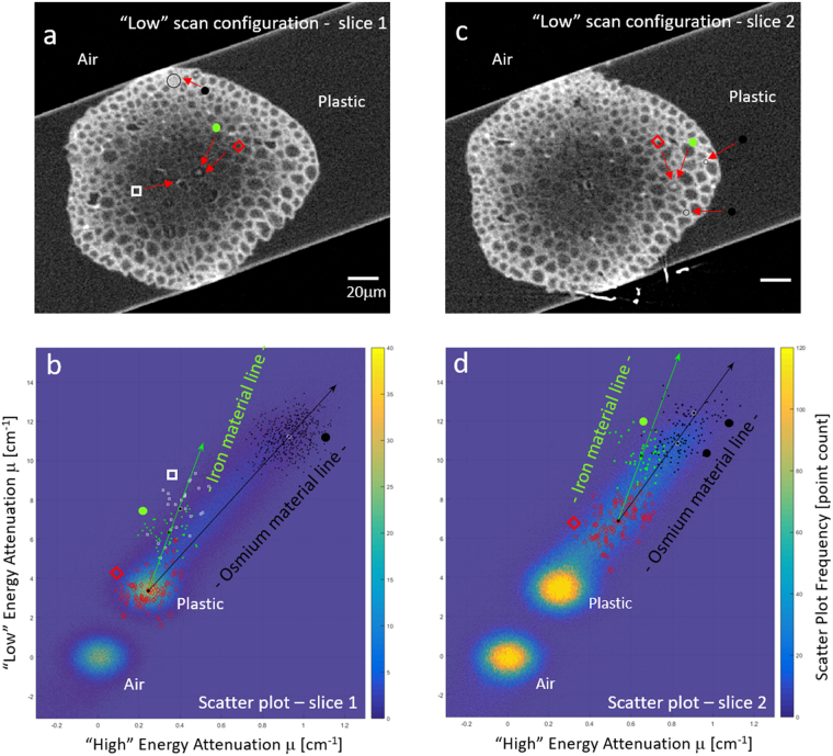
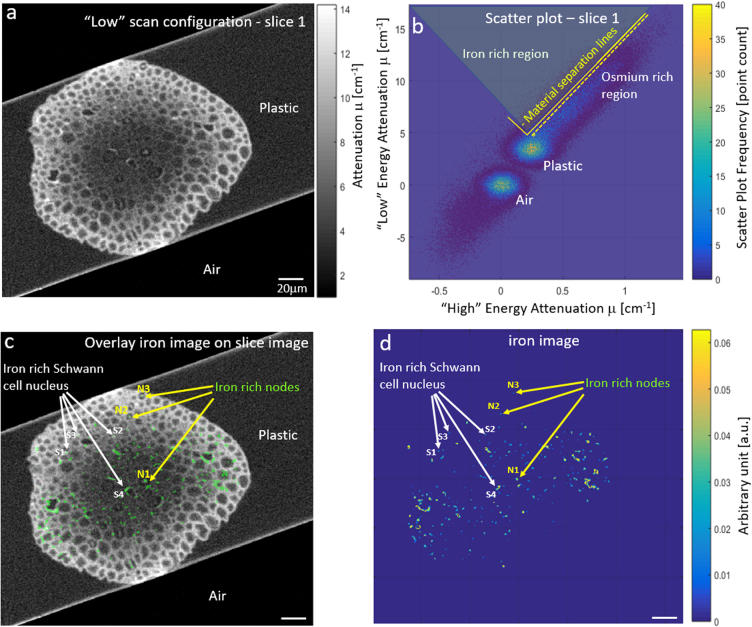
Biological samples are frequently stained with heavy metals in preparation for examining the macro, micro and ultra-structure using X-ray microtomography and electron microscopy. A single X-ray microtomography scan reveals detailed 3D structure based on staining density, yet it lacks both material composition and functional information. Using a commercially available polychromatic X-ray source, energy integrating detectors and a two-scan configuration labelled by their energy- "High" and "Low", we demonstrate how a specific element, here shown with iron, can be detected from a mixture with other heavy metals. With proper selection of scan configuration, achieving strong overlap of source characteristic emission lines and iron K-edge absorption, iron absorption was enhanced enabling K-edge imaging. Specifically, iron images were obtained by scatter plot material analysis, after selecting specific regions within scatter plots generated from the "High" and "Low" scans. Using this method, we identified iron rich regions associated with an iron staining reaction that marks the nodes of Ranvier along nerve axons within mouse spinal roots, also stained with osmium metal commonly used for electron microscopy.

Figure 1

“High” and “Low” scan configuration of a phantom containing uranium and iron aqueous solutions in microtubes. Material analysis is performed in the middle row by scatter plot material analysis and in the last row by material basis decomposition. (a) 3D volume rendering of phantom configuration. (b,c) “High” and “Low” scan slice image, at 60 kVp with 25 μm thick iron filter and 30 kVp without filtration respectively. Material concentration in [%] by weight of compound, ferric chloride or uranyl acetate, are marked in (b). Water filled microtube and air were used to calibrate the results to give values in attenuation units [cm⁻¹]. (d) Scatter plot of “Low” vs. “High” pixel values showing “clouds” of distinct chemical composition. (e,f) Scatter plot material analysis of iron and uranium using (d), which after calibration result in density images in units of [mgFe/cc.] and [mgU/cc] for iron and uranium respectively. (g,h) Material basis decomposition results for iron and uranium.

Figure 2

X-ray characteristic emission spectrum and mass attenuation coefficient (energy) curves for several scan configurations and elements of interest. To create a strong elemental contrast, you need both cases of enhancement and suppression of Emission-absorption overlap. Source characteristic emission L-lines and location of iron K-edge onset at lower energy are used to enhance iron absorption. (a) Mass density attenuation coefficient (energy) curves $\mu /\rho [c{m}^2/g]$ for osmium (Os), lead (Pb), uranium (U) and iron (Fe) are plotted in logarithmic scale on the left y-axis. Iron is in dashed curve while all the other are solid line curves with the element symbol located at the edge onset. Measured X-ray emission spectrum [photon count] are plotted in the lower part of the graph using the right y-axis, showing two scan configurations, “Low” 30 kVp unfiltered and “High” 30 kVp filtered with 25 μm thick iron foil. “High” energy spectrum was scaled x1.8. The peak tube potential can be identified by the cuff-off energy of the spectrum. (b) Includes, iodine mass attenuation coefficient and third scan configuration, “High-2” 60 kVp filtered with 25 μm thick tungsten foil. Some of the other curves have been fainted out for clarity. “High-2” energy spectrum was scaled x2. The two scans “High” and “High-2” are pre- and post- iodine K-edge enhancing iodine contrast - a second potential marker.

Figure 3

Calculated absorption scatter/slope plot of various metals present in the sample using the “Low” – (30 kVp peak tube potential and no filtration) and “High”- (30 kVp peak tube potential and 25 μm thick iron filter) scan configurations. The separation capacity is a measure of ease of separation of two elements, proportional to the depicted perpendicular distance between the two slopes. The steeper slope for iron indicated it has the potential to be separated from the other metals.

Figure 4

Experimental XRM images of a mouse spinal root, stained with iron and osmium. (a,b) “Low” and “High” energy cross sectional images of spinal root, respectively. Red arrow points to location of node of Ranvier at center of red circle, specifically stained with iron. The circular structures are myelin sheaths stained with osmium. Air and plastic regions were used to calibrate. To ease comparison each image grayscale was set in the range [min, max] = [0, 4x (plastic value)]. In (b), air and plastic regions have been labeled. (c,d) Sagittal and coronal cross sections. Both images (a,b) are cross sections located at position of dashed line labeled slice 1. Images of cross section labeled slice 2 will be discussed in next figure. Enlargements of boxed regions around the marked node (c1-d1) are inserted in each. Scale bars are all 20 μm.

Figure 5

Scatter plots of the spinal root sample. Scatter plots (b,d) were generated by mapping each pixel by its “High” and “Low” attenuation value. Regions within the scatter plot can be traced to specific regions in the slice images shown in (a,c). Slice 1 (a) exemplifies a node in a low staining background. Two large point densities in the scatter plot are associated with air and plastic regions. A node (green circle) and another bright spot (white square) project in the scatter plot at a slope characteristic of iron, as seen when individual pixels associated with ROI are marked similarly in the scatter plot. Background locations with no prominent staining (red diamonds) were taken from the circular dark ring around the node and are associated with plastic. Myelin (black circles) ROI project along a line with a slope characteristic for osmium. Slice 2 (c) exemplifies a node in a region with considerable osmium staining, and so the iron is projected in the scatter plot (d) from a location already exhibiting some given osmium concentration.

Figure 6

Scatter plot was used to automatically segment the iron rich nodes of Ranvier regions. Other regions stained with iron were found out to be iron staining of the Schwann cell nucleus. (a) Slice image (b) Scatter plot allowing material analysis using shown material separation lines. (c) Overlay of Material analysis iron image (green) on original slice image. (d) Iron image proportional to iron density, in arbitrary units. All scale bars are 20 μm.

Figure 7

TEM and EELS measurements at the node of Ranvier and at a nearby control region. (a) TEM image showing staining of the node. EELS spectrum taken at the node showing strong presence of iron (b1) and osmium (b2) for which edge onset occurs at 708 eV and 1960eV, respectively. (c) EFTEM iron map confirms iron presence at the node (d) TEM of a control region showing a nearby axon of larger diameter. EELS spectrum taken at the control region showing the absence of iron (e1) yet presence of osmium at similar levels seen at the node (e2). (f) EFTEM iron map showing signal at noise level indicating the absence of iron in the control region. Scale bar for all images is 1 μm.

References

1. Metscher BD. Biological applications of X-ray microtomography: imaging micro- anatomy, molecular expression and organismal diversity. Microsc. Anal. 2013;27:13–16.
1. Mizutani R, Suzuki Y. X-ray microtomography in biology. Micron. 2012;43:104–115. doi: 10.1016/j.micron.2011.10.002. - DOI - PubMed
1. Bushong EA, et al. X-ray Microscopy as an Approach to Increasing Accuracy and Efficiency of Serial Block-face Imaging for Correlated Light and Electron Microscopy of Biological Specimens. Microsc. Microanal. 2015;21:231–238. doi: 10.1017/S1431927614013579. - DOI - PMC - PubMed
1. Ng, J. et al. Genetically targeted 3D visualisation of Drosophila neurons under Electron Microscopy and X-Ray Microscopy using miniSOG. Nat. Publ. Gr. 1–14, 10.1038/srep38863 (2016). - PMC - PubMed
1. Adams SR, et al. Multicolor Electron Microscopy for Simultaneous Visualization of Multiple Molecular Species. Cell Chem. Biol. 2016;23:1417–1427. doi: 10.1016/j.chembiol.2016.10.006. - DOI - PMC - PubMed
Publication types