Group Analysis in FieldTrip of Time-Frequency Responses: A Pipeline for Reproducibility at Every Step of Processing, Going From Individual Sensor Space Representations to an Across-Group Source Space Representation

Abstract

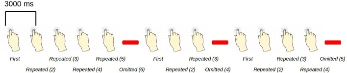
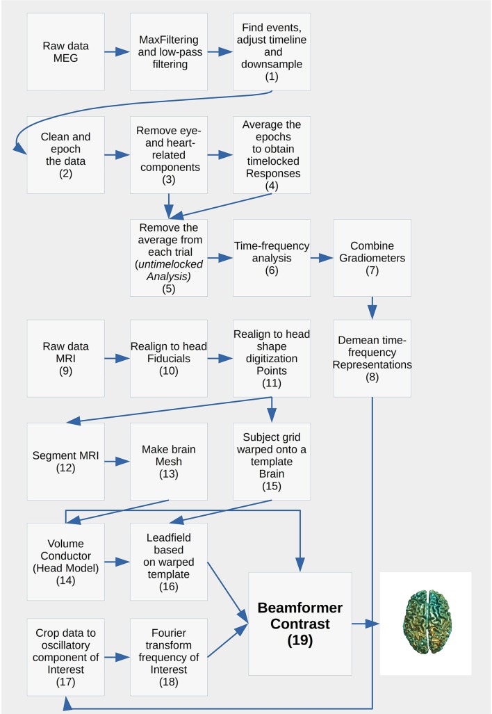
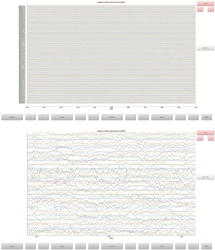
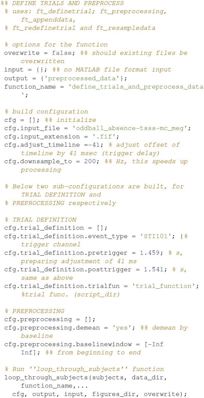
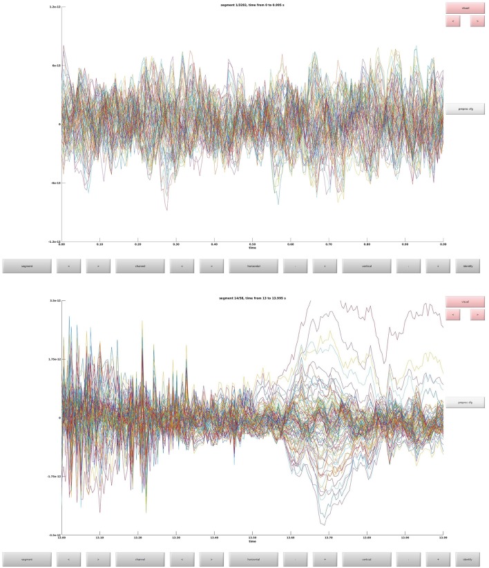
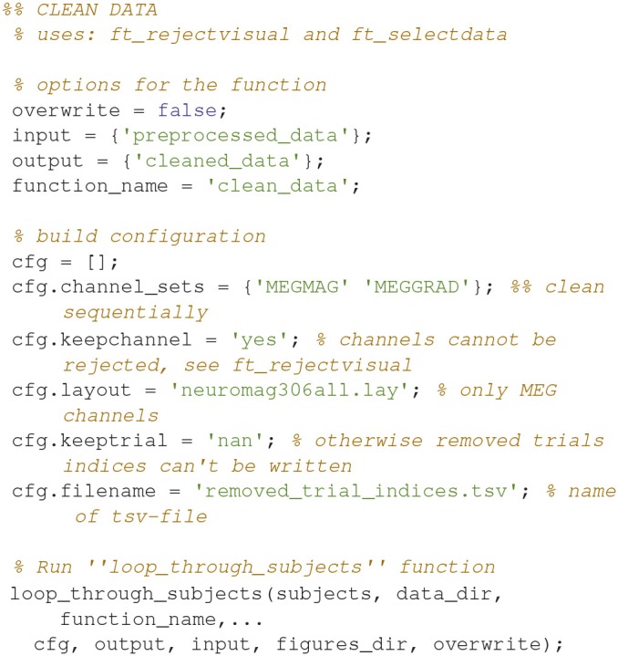
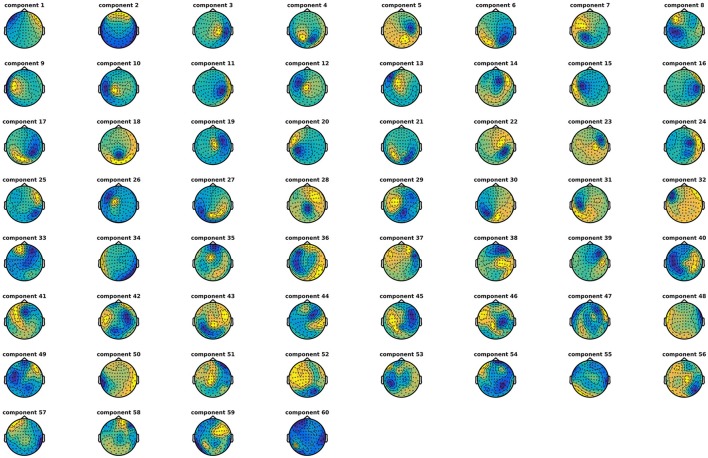
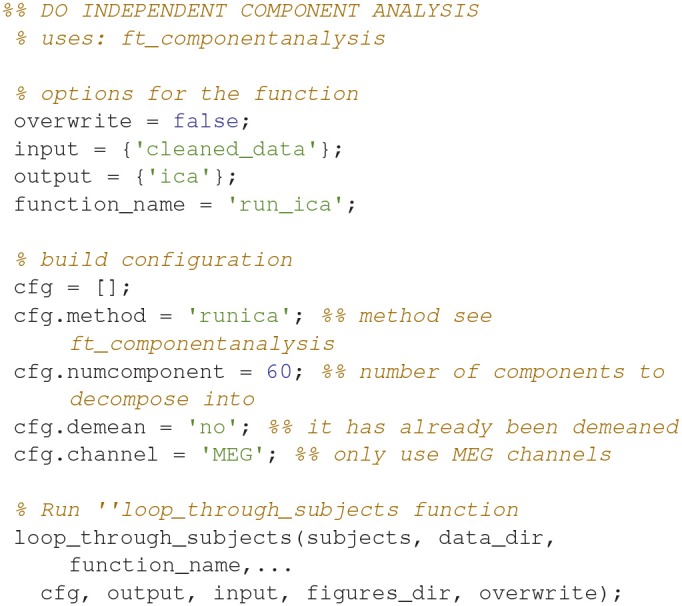
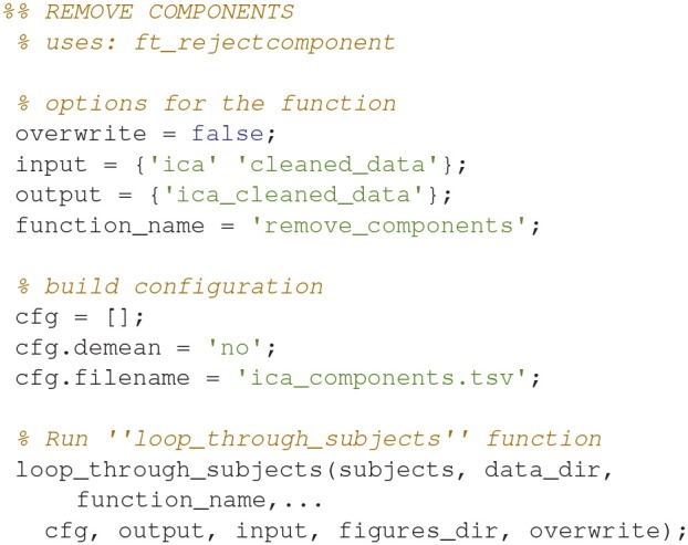
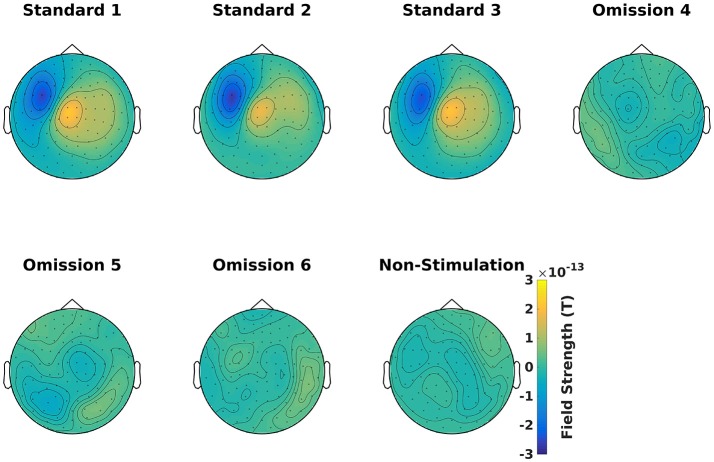
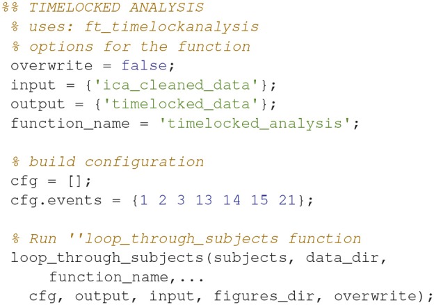
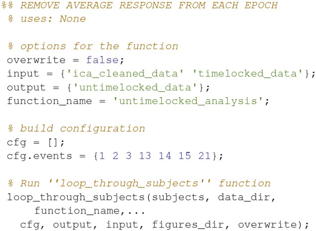
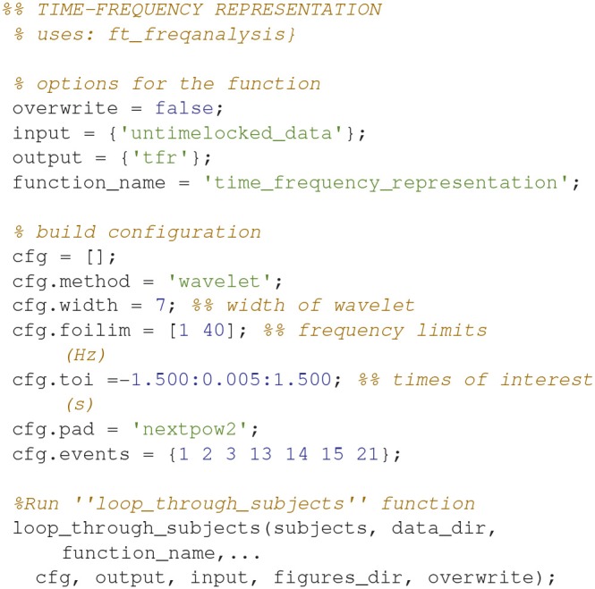
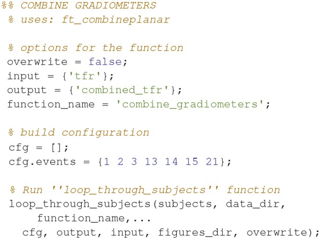
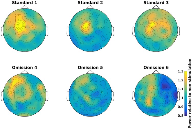
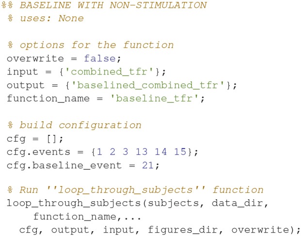
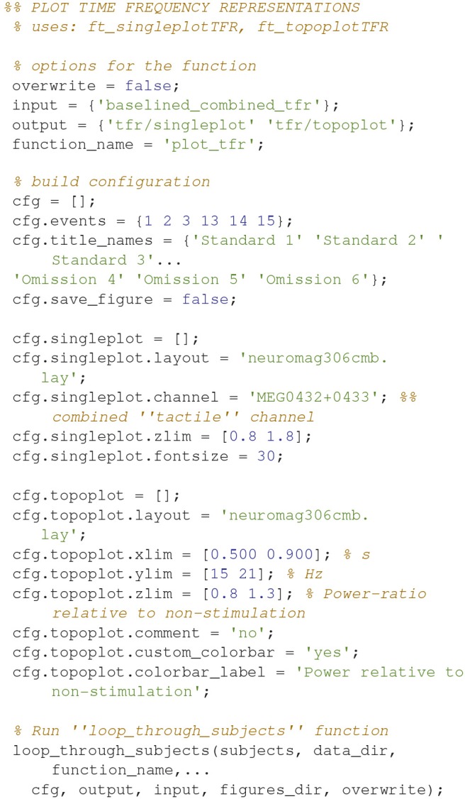
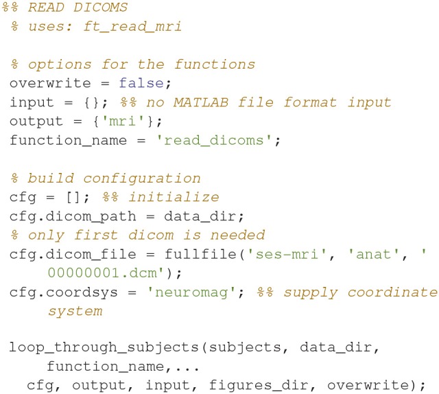
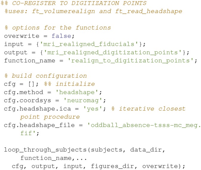
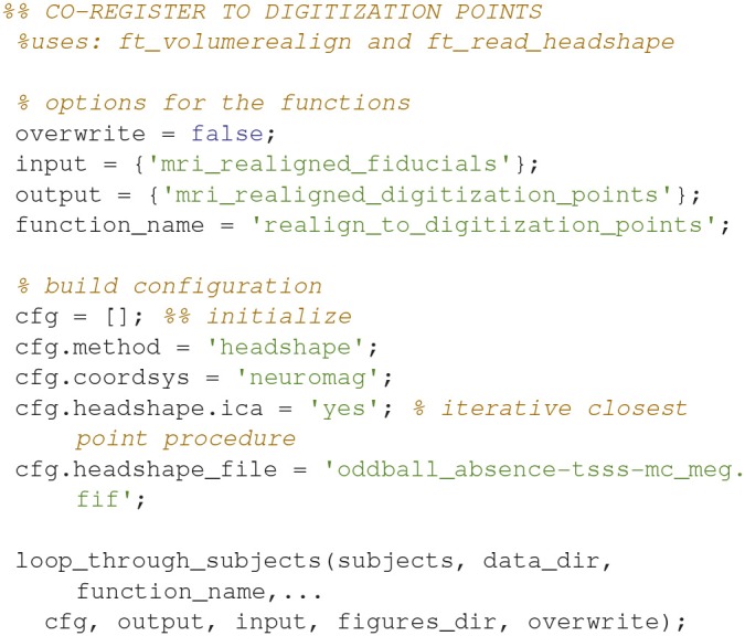
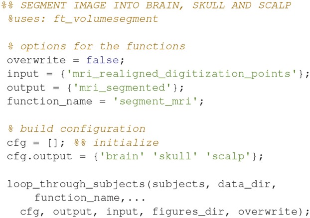
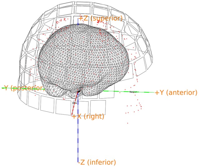
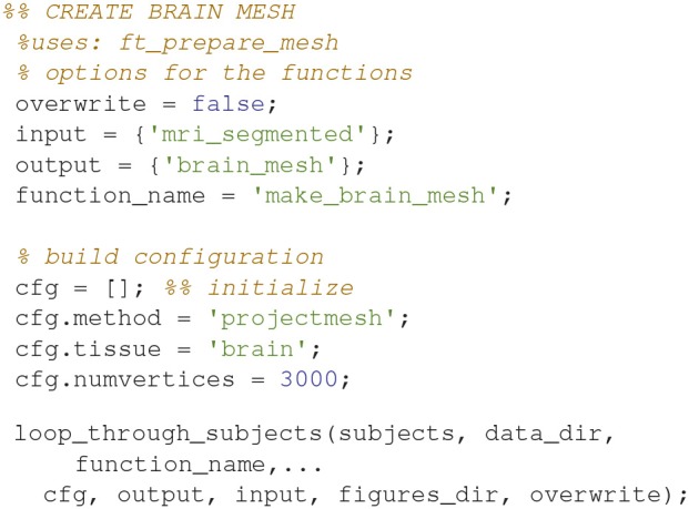
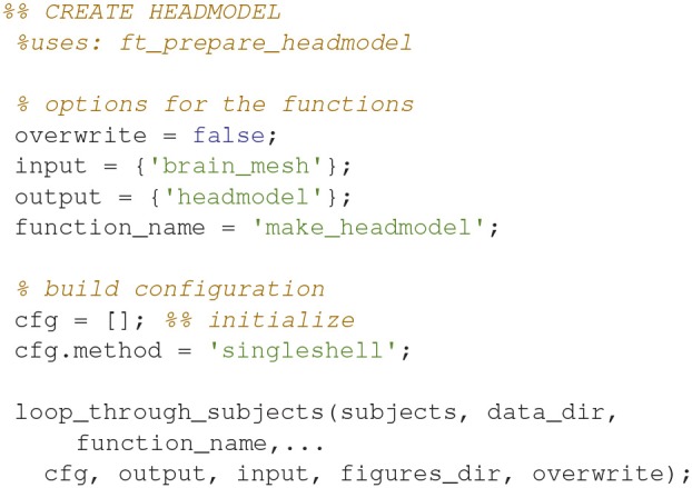
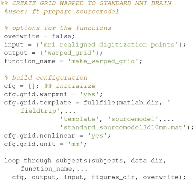
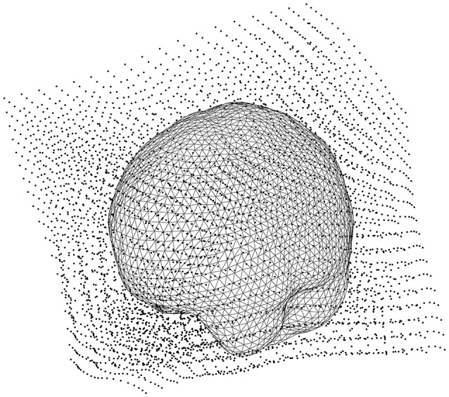
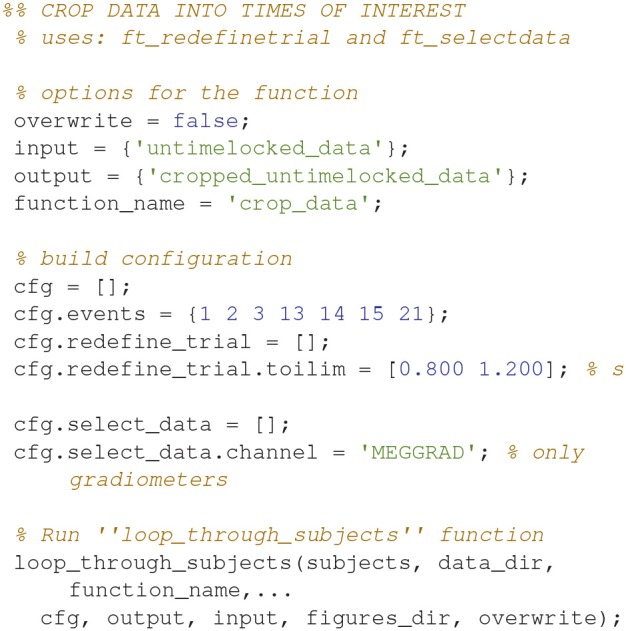
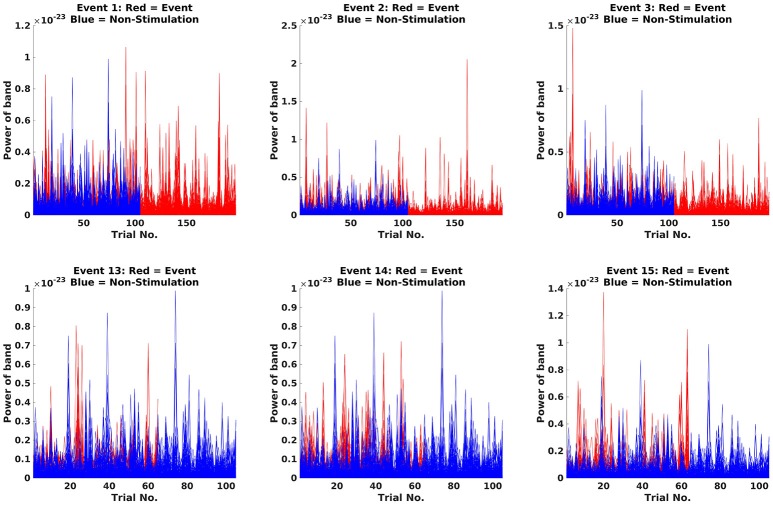
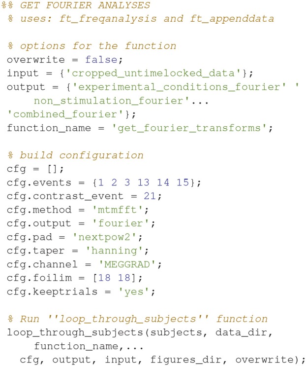
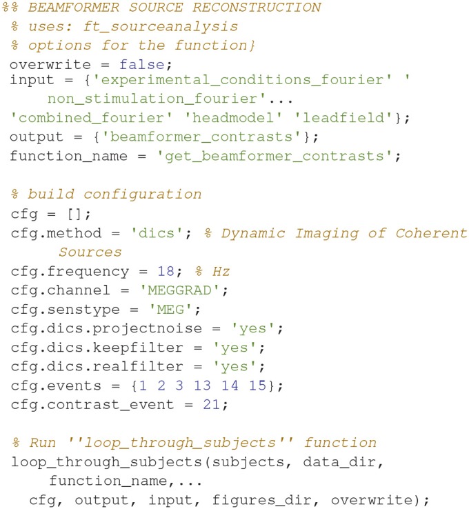
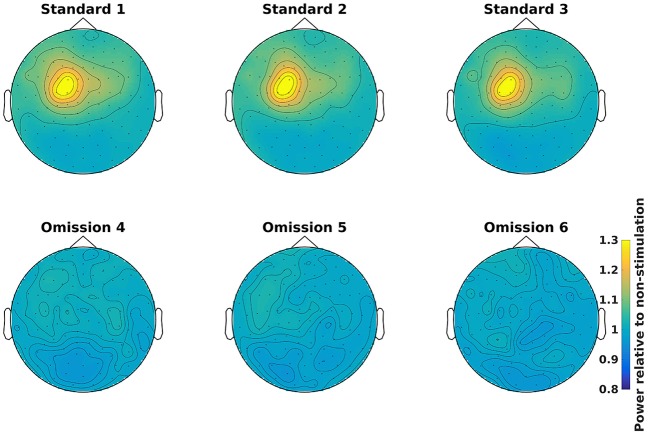
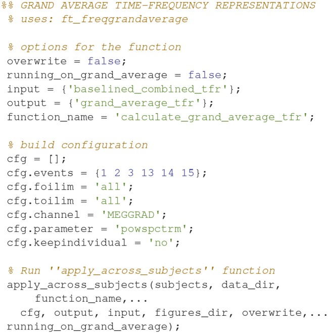
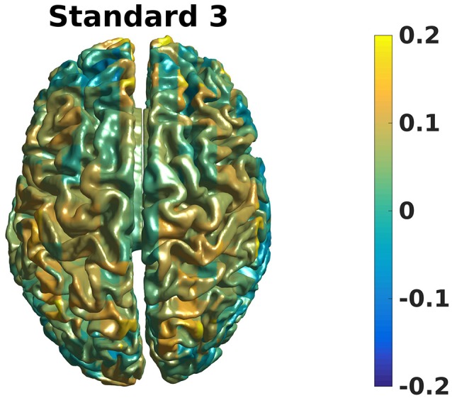
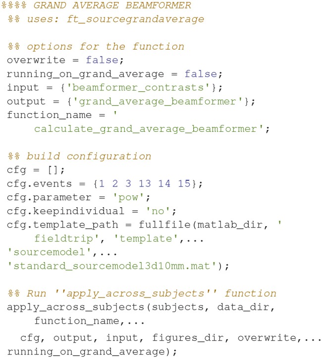
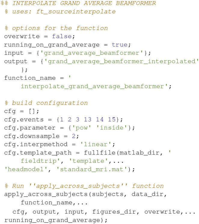
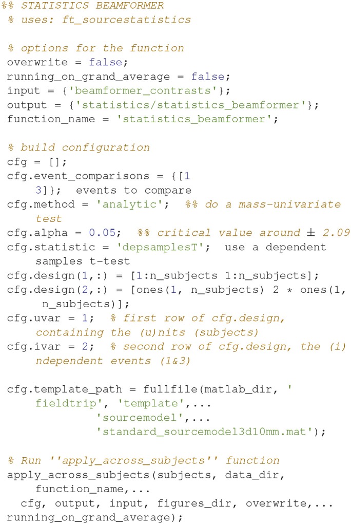
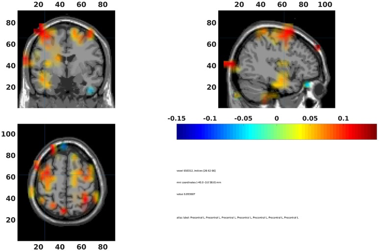
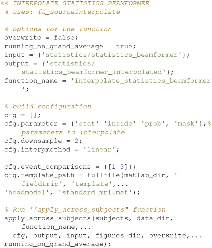
An important aim of an analysis pipeline for magnetoencephalographic (MEG) data is that it allows for the researcher spending maximal effort on making the statistical comparisons that will answer his or her questions. The example question being answered here is whether the so-called beta rebound differs between novel and repeated stimulations. Two analyses are presented: going from individual sensor space representations to, respectively, an across-group sensor space representation and an across-group source space representation. The data analyzed are neural responses to tactile stimulations of the right index finger in a group of 20 healthy participants acquired from an Elekta Neuromag System. The processing steps covered for the first analysis are MaxFiltering the raw data, defining, preprocessing and epoching the data, cleaning the data, finding and removing independent components related to eye blinks, eye movements and heart beats, calculating participants' individual evoked responses by averaging over epoched data and subsequently removing the average response from single epochs, calculating a time-frequency representation and baselining it with non-stimulation trials and finally calculating a grand average, an across-group sensor space representation. The second analysis starts from the grand average sensor space representation and after identification of the beta rebound the neural origin is imaged using beamformer source reconstruction. This analysis covers reading in co-registered magnetic resonance images, segmenting the data, creating a volume conductor, creating a forward model, cutting out MEG data of interest in the time and frequency domains, getting Fourier transforms and estimating source activity with a beamformer model where power is expressed relative to MEG data measured during periods of non-stimulation. Finally, morphing the source estimates onto a common template and performing group-level statistics on the data are covered. Functions for saving relevant figures in an automated and structured manner are also included. The protocol presented here can be applied to any research protocol where the emphasis is on source reconstruction of induced responses where the underlying sources are not coherent.

Keywords: MEG; analysis pipeline; beamformer; fieldtrip; good practice; group analysis; tactile expectations.

Figure 1

An example sequence of the experimental paradigm is shown. The annotations on the bottom show the coding used throughout for the different events of interest. Stimulations happened at a regular pace, every 3 s. When omissions occurred, there were thus 6 s between two consecutive stimulations.

Figure 2

Cookbook for performing a single subject analysis. Numbers point to the sections below.

Code Snippet 1

SET PATHS, ADD PATHS, and SUBJECTS AND DATES sections which are used to set up all analysis scripts.

Code Snippet 2

The loop_through_subjects function. This function is used to specify input (names), output (names), the function that take the input, the configuration that should be fed to the function. This is applied to all subject recordings in subjects_and_dates. Configurations (cfg) to FieldTrip functions can be used to easily change how the function is applied.

Figure 3

(Top) The raw data browser for the example subject. (Bottom) A zoom in on some sensors.

Code Snippet 3

Code for defining trials from raw data and preprocessing data.

Figure 4

(Top) The data browser showing the epoched data. A butterfly plot showing all the magnetometers. Here the first epoch is shown. (Bottom) The data browser showing all the magnetometers from one of the removed bad trials.

Code Snippet 4

Code for cleaning the preprocessed data.

Figure 5

The components found from the independent component analysis.

Code Snippet 5

Code for decomposing the data into independent components.

Code Snippet 6

Code for removing the components entered into ica_components.tsv from the epoched data.

Figure 6

Magnetometer topographical plots for averages from 50 to 70 ms, showing a dipolar pattern typical for activation of the somatosensory cortex. Scale is the same for all plots.

Code Snippet 7

Code for averaging the epochs.

Code Snippet 8

Code for removing the averaged response from each epoch.

Code Snippet 9

Code for calculating the time-frequency representation for each condition.

Code Snippet 10

Code for combining the gradiometer data in the time-frequency representation.

Figure 7

Power topographical plots for Standards and Omissions (baselined with Non-Stimulation) based on gradiometers averaged over 500 to 900 ms and 15 to 21 Hz (the beta rebound). Scale is the same for all plots.

Code Snippet 11

Code for demeaning the time-frequency representation with the non-stimulation time-frequency representation.

Code Snippet 12

Example code for creating plots of single sensors (not shown here) and topographies (Figure 7) for time-frequency representations. Creating and saving plots for each subject is also done with loop_through_subjects.

Code Snippet 13

Code for creating an MRI-structure based on reading in the dicoms.

Code Snippet 14

Code for opening the interactive alignment tool for aligning MRI with fiducials.

Code Snippet 15

Code for opening the interactive alignment tool for further aligning the fiducial-aligned MRI with the extra head shape digitization points acquired with the Polhemus Fastrak.

Code Snippet 16

Code for segmenting the brain into the three tissue types: brain, skull and scalp.

Figure 8

Quality control figure showing the brain, the digitization points, the sensors and the axes. This figure indicates if the realignment process has gone well. More quality figure checks are included in the pipeline.

Code Snippet 17

Code for preparing a brain mesh out of the segmented MRI.

Code Snippet 18

Code for making a head model (volume conductor) out of the prepared brain mesh.

Code Snippet 19

Code for making a grid where the subject's MRI is warped onto a template brain.

Figure 9

The head model (volume conductor) inside the grid that has been warped to a common template.

Code Snippet 20

Code for calculating the lead field (forward model) for all the sources of the warped grid that are contained by the brain.

Figure 10

(Top) Grand average multiplot masking the non-significant parts. Color shows where there is more/less power for Standard 1 when compared to Standard 3. Red square indicates the sensor shown below. (Bottom) Difference in the beta rebound. This is chosen for the subsequent beamformer analysis.

Code Snippet 21

Code for calculating the statistics for the time-frequency representations.

Figure 11

The epochs in the beta rebound where they differ between novel and repeated stimulation (800–1,200 ms). It can be seen that there is no clear timelocked activity.

Code Snippet 22

Code for cropping the epoched data into the time window of interest.

Figure 12

Fourier transforms. On the y-axis, power is illustrated, and the x-axis shows the trials. For the Standards (red), it can be seen that the power is greater than for Non-Stimulations (blue).

Code Snippet 23

Code for calculating the fourier transforms.

Code Snippet 24

Code for calculating the beamformer solutions based on the Fourier transforms and contrasting them against the non-stimulation cross-spectral density.

Figure 13

Grand average power topographical plots for Standards and Omissions (baselined with Non-Stimulation) based on gradiometers averaged over 500 to 1,400 ms and 15 to 21 Hz (the beta rebound). Scale is the same for all plots.

Code Snippet 25

Code for calculating the grand averages for time-frequency representations.

Figure 14

Grand average beamformer contrast. Color shows where there is more/less power for Standard 3 when compared to Non-Stimulation. (0 means equal power, and 0.2 means 20% more power).

Code Snippet 26

Code for calculating the grand averages for the beamformer source reconstructions.

Code Snippet 27

Code for interpolating the beamformer source reconstructions onto a common template.

Code Snippet 28

Code for calculating the statistics for the beamformer source reconstructions.

Figure 15

Grand average beamformer interpolated onto a common template and non-significant voxels assigned no color. Colors indicate difference between Standard 1 and Standard 3. The cross-hair is centered on the contralateral motor cortex. Ipsilateral activation is also seen in the motor cortex.

Code Snippet 29

Code for interpolating the beamformer statistics onto a common template.

References

1. Cheyne D. O. (2013). MEG studies of sensorimotor rhythms: a review. Exp. Neurol. 245, 27–39. 10.1016/j.expneurol.2012.08.030 - DOI - PubMed
1. Dalal S. S., Baillet S., Adam C., Ducorps A., Schwartz D., Jerbi K., et al. . (2009). Simultaneous MEG and intracranial EEG recordings during attentive reading. Neuroimage 45, 1289–1304. 10.1016/j.neuroimage.2009.01.017 - DOI - PubMed
1. Gaetz W., Cheyne D. (2006). Localization of sensorimotor cortical rhythms induced by tactile stimulation using spatially filtered MEG. Neuroimage 30, 899–908. 10.1016/j.neuroimage.2005.10.009 - DOI - PubMed
1. Gaetz W., MacDonald M., Cheyne D., Snead O. C. (2010). Neuromagnetic imaging of movement-related cortical oscillations in children and adults: age predicts post-movement beta rebound. Neuroimage 51, 792–807. 10.1016/j.neuroimage.2010.01.077 - DOI - PubMed
1. Galan J. G. N., Gorgolewski K. J., Bock E., Brooks T. L., Flandin G., Gramfort A., et al. (2017). MEG-BIDS: an extension to the brain imaging data structure for magnetoencephalography. bioRxiv 172684. 10.1101/172684 - DOI
LinkOut - more resources