Digital Museum of Retinal Ganglion Cells with Dense Anatomy and Physiology

Abstract

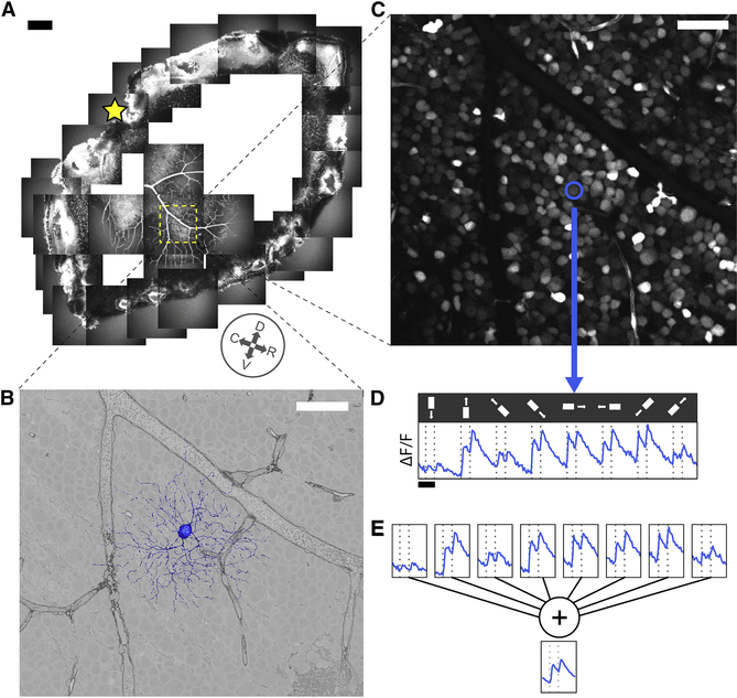
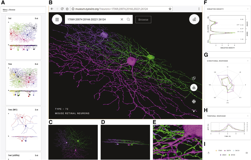
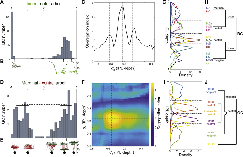
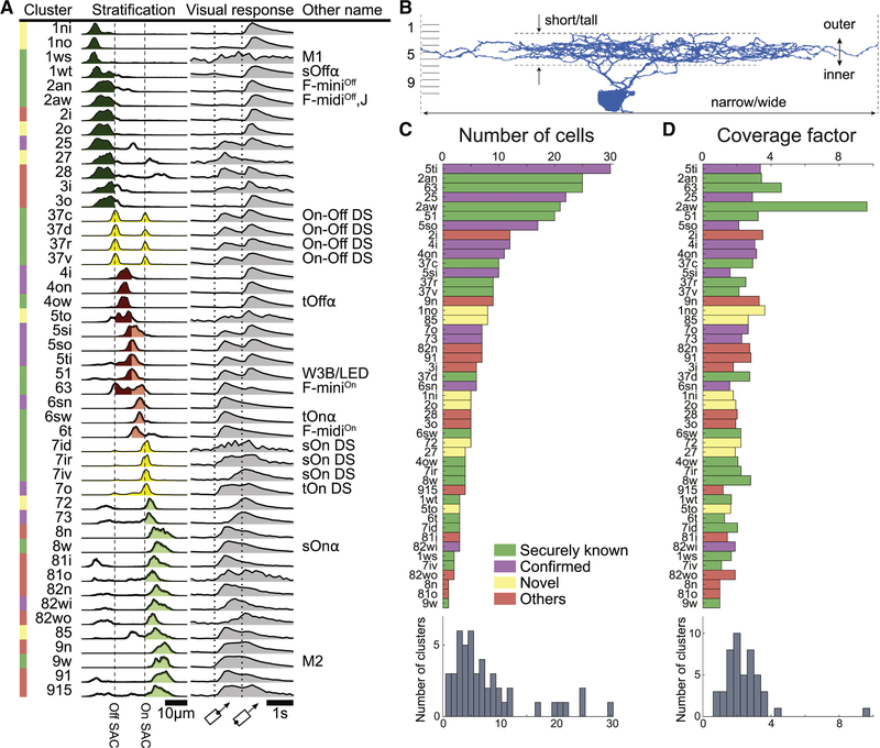
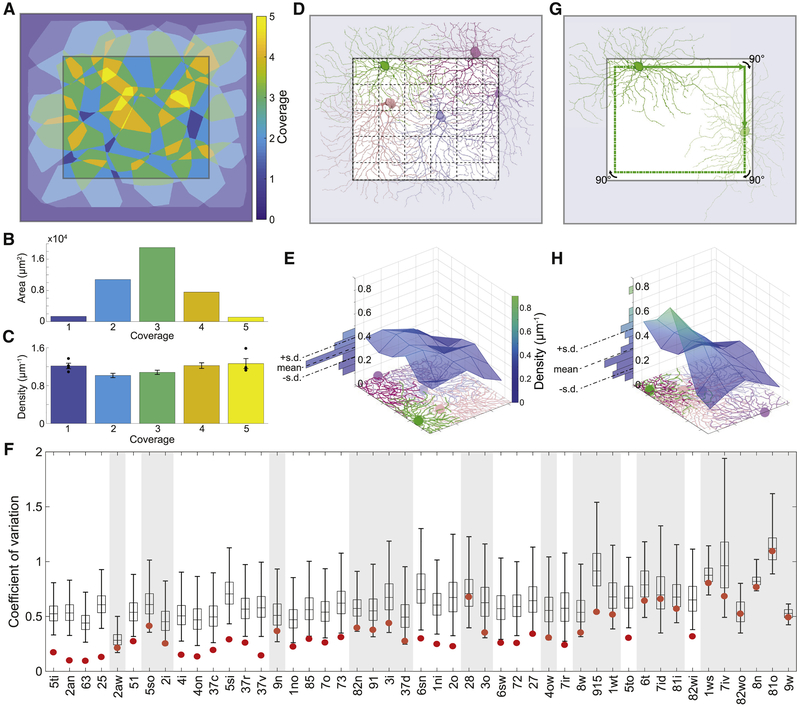
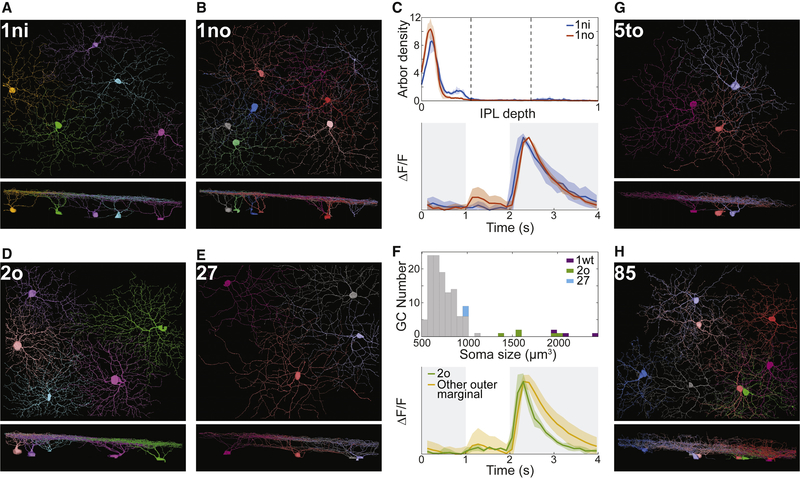
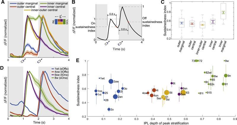
When 3D electron microscopy and calcium imaging are used to investigate the structure and function of neural circuits, the resulting datasets pose new challenges of visualization and interpretation. Here, we present a new kind of digital resource that encompasses almost 400 ganglion cells from a single patch of mouse retina. An online "museum" provides a 3D interactive view of each cell's anatomy, as well as graphs of its visual responses. The resource reveals two aspects of the retina's inner plexiform layer: an arbor segregation principle governing structure along the light axis and a density conservation principle governing structure in the tangential plane. Structure is related to visual function; ganglion cells with arbors near the layer of ganglion cell somas are more sustained in their visual responses on average. Our methods are potentially applicable to dense maps of neuronal anatomy and physiology in other parts of the nervous system.

Keywords: 3D reconstruction; calcium imaging; cell type; crowdsourcing; electron microscopy; ganglion cell; inner plexiform layer; mouse; online atlas; retina.

Figure 1:. Anatomy and Physiology of Retinal Ganglion Cells via Electron and Light Microscopy.

(A) Hemiretina containing imaged 0.3×0.35 mm² patch (yellow square). Star, optic disk. Compass rosette, inferred cardinal directions (dorsal, ventral, rostral, caudal, see Methods). (B) 3D reconstruction of GC dendritic arbor (blue) and 2D cross section through GCL in serial EM image (grayscale). (C) Soma of same GC (blue) in image of GCL obtained via two-photon microscopy. (D) Fluorescence versus time for same GC along with stimulus sequence of light bar moving in eight directions on dark background (0.2 mm×1 mm). (E) Averaging over stimulus directions (shown) and trials (not shown) yields temporal response function for GC. Scale bars, 200 μm (A), 50 μm (B, C) and 2 sec (D).

Figure 2:. Eyewire Museum (museum.eyewire.org).

(A) Left collapsible sidebar enables browsing GC clusters. (B) Display of 3D rendering of selected cells. URL containing the cell IDs can be shared. (C) View along the light axis (“whole mount” view) of the retina. (D) View along the tangential axis. (E) Zoomed-in view. (F-H) Anatomical and physiological properties included in right collapsible sidebar; stratification profiles (F), directional response (G), and temporal response (H). (I) Right collapsible sidebar shows a list of selected cells. Mousing over a cell ID highlights the cell and its properties and cells can be removed from the display.

Figure 3:. Maximizing Laminar Segregation of Arbors Yields Marginal-Central and Inner-Outer Divisions of the IPL.

(A) Histogram of the difference between inner and outer arbor volume for BCs (total volume normalized to one). BC axonal arbors are either mostly inner (right cluster) or mostly outer (left cluster); intermediate cases are rare. (B) Inner arbor (light green) and outer arbor (dark green) of example BCs. The depth of the inner-outer boundary is denoted by d₀. (C) BC inner-outer segregation is maximized for d₀ = 0.47 (dotted line, same value used in A), with two flanking local maxima at or near the SAC depths (dashed lines). (D) Histogram of the difference between marginal and central arbor length for GCs (total length normalized to one). GC dendritic arbors are either mostly marginal (right bump) or mostly central (left bump). The segregation index is defined as the separation between the clusters (dashed line), divided by the square root of the average of the half widths of the clusters (full widths are solid lines). (E) Marginal arbor (green) and central arbor (red) of example GCs (aspect ratio of the cells are distorted for visualization). The IPL depths of the marginal-central boundaries are denoted by d₁ and d₂. (F) GC marginal-central segregation index is maximized for d₁ and d₂ at the SAC depths (dashed lines, same values used in D). (G) Average stratification profiles (linear density of arbor volume vs. IPL depth) of BC types. (H) BC types belong to four high-level BC clusters created by inner-outer and marginal-central splits. (I) Average stratification profiles (linear density of arbor length vs. IPL depth) of six high-level GC clusters. (J) High-level hierarchical clustering of GCs. See also Figure S1.

Figure 4:. Classification of Ganglion Cells.

(A) Summary of clusters with anatomical name, stratification profile, and temporal response function defined in Fig. 1E. Alternative names in black are “securely known” types (see main text for definition). (B) Each cluster name begins with a number in the range 1–9 indicating which tenth of the IPL depth contains the most stratification profile area. More numbers are appended for multistratified clusters. Letters (s, t, n, w, o, i, a) are added to distinguish between clusters with similar stratification, where “a” denotes asymmetric arbor. (C) Number of cells in each cluster. (D) Coverage factors. See also Figures S2, S3, S4, S5, and S6.

Figure 5:. According to Our Density Conservation Principle, the Arbors of a GC Type Should Have an Aggregate Density that is Approximately Uniform.

(A) Arbor convex hulls of an example cluster (25) overlap substantially. Colors indicate how many hulls cover each retinal location inside the crop region. (B) Retinal area versus coverage inside the crop region. Each bar represents the area devoted to the corresponding color/coverage in the crop region. (C) The aggregate arbor density of the cluster varies relatively little with coverage. Each bar represents the density within the area devoted to the corresponding color/coverage in the crop region (standard error, n = 4, 19, 33, 20, 4). (D) The crop region is divided into grid boxes, and the aggregate arbor density is computed for each box, as illustrated for an example cluster (6sw). (E) The aggregate arbor density is close to uniform across the crop region, as quantified by the coefficient of variation (standard deviation divided by mean). (F) The density conservation test is satisfied by a cluster (non-shaded) when the coefficient of variation is significantly smaller for the real configuration (red dot) than for 99% of all randomized configurations (99/1 percentiles, black bar; quartiles and median, box; n = 10,000). (G) To test statistical significance, the arbors of a cluster are randomized by relocating the soma somewhere on its “orbit” (green line) and rotating the arbor to have the same orientation relative to the nearest side of the retinal patch. (H) The aggregate arbor density typically varies more after randomization. Example cluster is 25 in A-C and 6sw in D, E, G, H.

Figure 6:. Novel Ganglion Cell Types, Views Along the Light Axis and a Tangential Axis.

(A-C) 1ni and 1no are types with very similar stratification profiles (C, top) and temporal response functions (C, bottom). (D-F) 2o and 27 are outer marginal types. Histogram of soma size for outer marginal cells shows that 2o somas are much larger than those of 27 and other typical cells, and smaller than 1wt (transient Off alpha) somas (F, top). The Off response of 2o decays more rapidly than that of other outer marginal cells (F, bottom). (G) 5to looks monostratified in the tangential view but its stratification profile (Fig. 4A) is surprisingly complex. (H) 85 stratifies throughout the inner IPL but also extends sparse branches towards the INL. Shaded regions around curves in C and F represent standard deviations.

Figure 7:. Sustainedness of Visual Responses and Dendritic Stratification.

(A) Average temporal response function (Fig. 1E) for high-level GC clusters (Fig. 3I). Each response function is averaged over cells in a cluster, and normalized to have the same maximum and minimum. The inner marginal cluster is markedly more sustained than the others. Shading indicates standard error (n = 102, 26, 78, 12, 55 for outer marginal, outer central, inner-outer central, inner central, inner marginal). (B) The sustainedness index is defined as the response at 0.8 s after nominal stimulus onset, divided by peak response in the 0.8 s interval. (C) The cells in the inner marginal cluster are significantly more sustained than cells in the other clusters (ANOVA with post hoc p < 0.01). The differences between other clusters are not statistically significant. Colored, mean and standard error; grey box and bars, quartiles, median, and extrema. (D) Marginal is more sustained than central for the four alpha types. Shading indicates standard error of the mean (n = 4, 5, 4 for 4ow, 6sw, 8w). There is no standard error for 1wt, because only a single 1wt cell had calcium signals. Applying t-tests to sustainedness indices yield p = 0.02 for 1wt against 4ow, and p = 0.03 for 8w against 6sw. (E) Sustainedness index for cells with high response quality (Methods, Eq. 4), sorted by clusters. Bars indicate standard deviations for the clusters, except for clusters containing only a single cell with high response quality (1wt, 28, 81i, 8n, 915, 9w). Dot area indicates the number of cells in the cluster; the largest dot (63) represents 18 cells. See Figure S7 for size-adjusted sustainedness index for individual cells.

References

1. Amunts K, Lepage C, Borgeat L, Mohlberg H, Dickscheid T, Rousseau M-É, Bludau S, Bazin P-L, Lewis LB, Oros-Peusquens A-M, et al. (2013). BigBrain: An ultrahigh-resolution 3D human brain model. Science, 340(6139):1472–1475. - PubMed
1. Arthur D and Vassilvitskii S (2007). k-means++: The advantages of careful seeding. In Proceedings of the 18th annual ACM-SIAM symposium on Discrete algorithms, pages 1027–1035. Society for Industrial and Applied Mathematics.
1. Ascoli GA, Donohue DE, and Halavi M (2007). NeuroMorpho.org: A central resource for neuronal morphologies. Journal of Neuroscience, 27(35):9247–9251. - PMC - PubMed
1. Awatramani GB and Slaughter MM (2000). Origin of transient and sustained responses in ganglion cells of the retina. J Neurosci, 20(18):7087–95. - PMC - PubMed
1. Badea TC and Nathans J (2004). Quantitative analysis of neuronal morphologies in the mouse retina visualized by using a genetically directed reporter. J Comp Neurol, 480(4):331–51. - PubMed
Publication types
LinkOut - more resources