In vivo wide-field calcium imaging of mouse thalamocortical synapses with an 8 K ultra-high-definition camera

Abstract

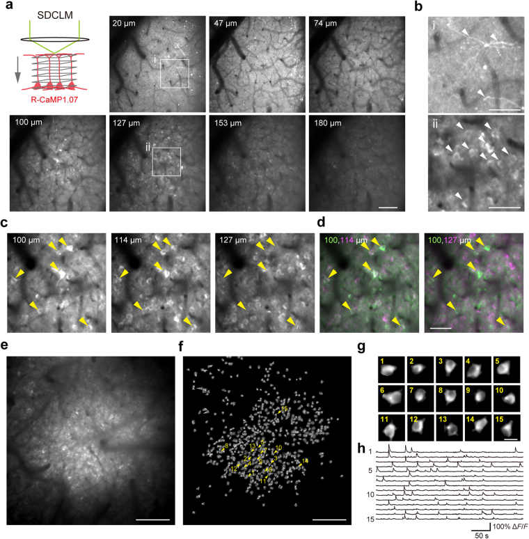
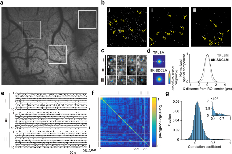
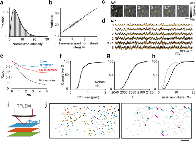
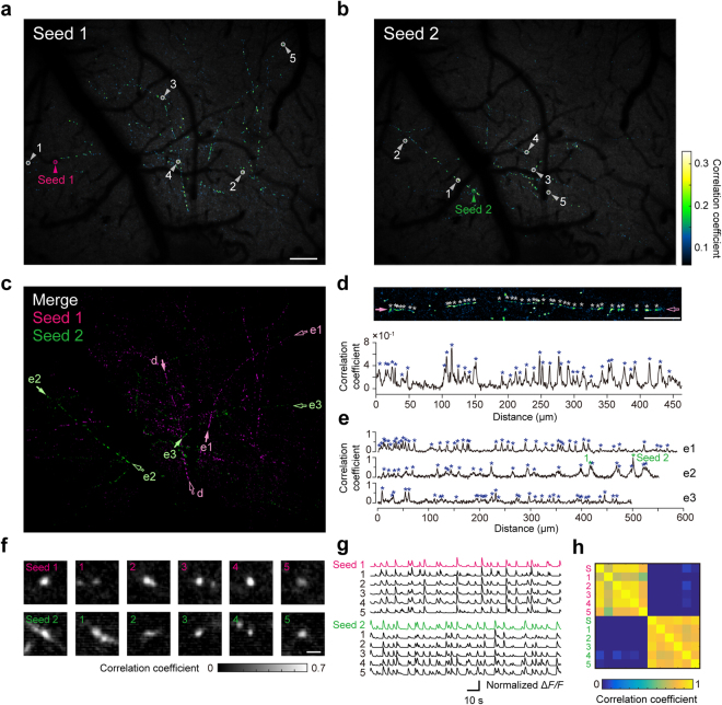
In vivo wide-field imaging of neural activity with a high spatio-temporal resolution is a challenge in modern neuroscience. Although two-photon imaging is very powerful, high-speed imaging of the activity of individual synapses is mostly limited to a field of approximately 200 µm on a side. Wide-field one-photon epifluorescence imaging can reveal neuronal activity over a field of ≥1 mm² at a high speed, but is not able to resolve a single synapse. Here, to achieve a high spatio-temporal resolution, we combine an 8 K ultra-high-definition camera with spinning-disk one-photon confocal microscopy. This combination allowed us to image a 1 mm² field with a pixel resolution of 0.21 µm at 60 fps. When we imaged motor cortical layer 1 in a behaving head-restrained mouse, calcium transients were detected in presynaptic boutons of thalamocortical axons sparsely labeled with GCaMP6s, although their density was lower than when two-photon imaging was used. The effects of out-of-focus fluorescence changes on calcium transients in individual boutons appeared minimal. Axonal boutons with highly correlated activity were detected over the 1 mm² field, and were probably distributed on multiple axonal arbors originating from the same thalamic neuron. This new microscopy with an 8 K ultra-high-definition camera should serve to clarify the activity and plasticity of widely distributed cortical synapses.

Figure 1

Optical performance of SDCLM. (a) Schematic principle of SDCLM. Arrayed microlenses split the excitation laser beam (green) and focus each of the split beams into its corresponding pinhole. The laser beam passing the pinhole focuses through the objective lens to the corresponding spot and excites fluorophores. Emitted fluorescence (red) passes the corresponding pinhole and focuses onto the corresponding photosensor. Each pinhole prevents out-of-focus fluorescence from reaching the corresponding photosensor. Right bottom panel, a representative image of non-rotating pinholes at the sample plane. Scale bar, 200 µm. (b) To measure the spatial resolution in SDCLM imaging (c,d), fluorescent beads were embedded in 0.5% agarose gel and Z-stacks of the beads located around a depth of 20 µm from the coverslip were acquired. (c) Representative normalized XY (left) and XZ (right) SDCLM images of fluorescent beads with a diameter of 0.5 µm. Scale bar, 2 µm. (d) The FWHMs of the 0.5 µm beads along X (top) and Z (bottom) axes (n = 5 for each axis). A Gaussian curve (blue) was fitted to the intensity profile of the bead along each axis. (e) Representative normalized XZ images of fluorescent beads with a diameter of 0.5 µm (bottom) at three locations along the X axial centerline in a 1 mm FOV (top). Scale bar, 5 µm. (f) Lateral and axial FWHMs and intensity of the 0.5 µm beads at six locations along the X axial centerline in the FOV (n = 5 beads for each point). The FWHMs at the center of the FOV were longer than those in d. This was probably because the pixel width of the camera image that was used to calculate the FWHMs was larger in f (1.05 µm at the sample) than in d (0.21 µm at the sample). (g–j) Performance of SDCLM compared with OEFM in a tissue phantom. (g) Tissue phantom preparation. Fluorescent beads with a diameter of 2.0 µm (green circles) were embedded in 0.5% agarose gel with non-fluorescent polystyrene beads (open circles) as a scattering agent, and were imaged with OEFM or SDCLM. Volumes of 1 × 1 × 0.3 mm were imaged at 2 µm spacing along the Z axis. (h) Representative images of the 2.0 µm fluorescent beads at two depths (top, 5 µm depth, and bottom, 210 µm depth) with OEFM (left) and SDCLM (right). The images were cropped (300 × 300 µm) from the original images (1 × 1 mm). Scale bar, 100 µm. (i) Signal-to-background ratios as a function of the imaging depth, where the signal was the maximum fluorescence intensity in a 30 × 30 µm square that had an in-focus fluorescent bead at the center and did not appear to have any other one, and the background was the average intensity of this square excluding a circle with a diameter of 10 µm at the center of the square. Data were presented as mean ± SEM. **p < 0.01, n = 5 beads, Wilcoxon rank sum test. (j) Axial resolution as a function of imaging depth. The values were normalized to the mean value at a 5 µm depth in the SDCLM image and plotted as mean ± SEM (n = 5 beads for each point). *p < 0.1, **p < 0.01, Wilcoxon rank sum test.

Figure 2

SDCLM imaging of in vivo R-CaMP1.07-expressing L2/3 neurons. (a) SDCLM imaging of R-CaMP1.07-expressing neurons at seven cortical depths in the somatosensory cortex. The images were cropped (500 × 500 µm) from the original images (1 × 1 mm). Each image was the average of 4 s of imaging at 25 fps. Scale bar, 100 µm. (b) Magnified images from depths of 20 µm (i) and 127 µm (ii) in a. Arrowheads indicate putative dendrites in i and neuronal somata in ii. Scale bars, 50 µm. (c) Magnified images from depths of 100, 114, and 127 µm in a. Yellow arrowheads indicate neuronal somata observed at 100 and 114 µm, but not at 127 µm. (d) Composite images from c. The green channel corresponds to the depth of 100 µm; the magenta channel corresponds to 114 µm in the left panel and 127 µm in the right panel. Scale bar, 50 µm. (e) SDCLM imaging of L2/3 neuronal somata that expressed R-CaMP1.07 in the motor cortex. The depth was 120 µm from the cortical surface. The image was the average projection during the entire imaging period (10,000 frames over 500 s). Scale bar, 200 µm. (f) All the spatial components in image e are extracted by the constrained non-negative matrix factorization algorithm. (g) Fifteen representative extracted spatial components. Each component corresponds to the arrowheads in f. Scale bar, 20 µm. (h) ΔF/F traces extracted from the neuronal somata corresponding to ROIs in g.

Figure 3

In vivo imaging of thalamocortical axonal boutons with TPLSM, OEFM, SDCLM, and 8K-SDCLM. (a) Schematic illustration of imaging of TC axons in L1. (b) Representative two-photon image of TC axons that expressed GCaMP6s. The image is the average projection during the imaging. The image was cropped (85 × 85 µm) from the original 127 × 127 µm acquisition. Scale bar, 20 µm. (c,e) Representative OEFM (c) and SDCLM (e) imaging of tdTomato-expressing TC axons in the same cortical field. Scale bars, 200 µm. (d,f) Magnified images of white boxes in c (d) and e (f). Scale bars, 20 µm. (g) 8K-SDCLM imaging of a TC axon that expressed GCaMP6s. The image is the mean projection of frames in which the frame-averaged fluorescence exceeded its time-average value plus 2S.D. Scale bar, 200 µm. (h) Magnified images of blue and orange boxes in g. Scale bars, 20 µm.

Figure 4

In vivo imaging of axonal boutons in a 1 mm² cortical area. (a) 8K-SDCLM image of the motor cortical area overlapping the imaging field shown in Fig. 3g. The imaging experiment was performed a day after the image shown in Fig. 3g was acquired. Three areas were randomly chosen for image processing with the CNMF algorithm (i,ii,iii). The length of one side was 213 µm. The size of each square corresponded to 1024 × 1024 pixels. Scale bar, 200 µm. (b) All spatial components extracted by the CNMF algorithm. (c) Representative merged images of the pseudocolored spatial components and mean projections of highly activated frames in which the frame-averaged fluorescence exceeded its time-average value plus 3S.D. Scale bar, 4 µm. (d) Left, averaged images of ROIs from the images obtained by TPLSM and 8K-SDCLM (TPLSM, 1653 ROIs from six imaging fields; 8K-SDCLM, 373 ROIs from the three 213 × 213 µm areas in a). Individual ROIs were aligned at the center, and the normalized spatial component of each pixel was averaged and pseudocolor coded. Scale bar, 2 µm. Right, profiles of the normalized spatial components of the averaged ROIs along the dotted lines shown in the left panels. (e) ΔF/F traces extracted from 30 ROIs numbered in b. (f,g) Matrix (f) and histogram (g) of pair-wise correlation coefficients of the activities of ROIs in b. The matrix was arranged according to the orders of hierarchal clusters, on the basis of pair-wise correlation coefficients. The histogram of the correlation coefficients showed a second peak around 0.6 (inset in g). The bin width is 0.02 (0.03 in inset).

Figure 5

Comparisons in detected ROIs and their activity between 8K-SDCLM and TPLSM imaging. (a) Representative distribution of the normalized fluorescence signals from one pixel in the field shown in Fig. 4ai (21,600 time points). The fitted gamma distribution is also shown (the shape parameter is 2.35 and scale parameter is 2.87). (b) Relationship between the variance and time-averaged normalized fluorescence signal for 100 pixels. The red cross indicates the pixel shown in a. The regression line is also shown (p = 1.81 × 10⁻⁷⁵, Pearson correlation test). (c) Representative 30 frame-averaged TPLSM images with the artificial noise (from left to right, NR = 0, 1, 2, 3, 3.71, and 5). The ROI area corresponding to the left-most one was extracted from each image and its contour was overlaid on each image. Scale bar, 5 µm. (d) ΔF/F traces of the ROI areas shown in c. Black traces were directly calculated from the fluorescence signals from the motion-corrected raw images with artificial noise. Orange traces were denoised traces obtained using the CNMF algorithm. (e) Ratios of the number of detected ROIs (black), the number of detected spike events (red), and the pair-wise correlation coefficients in the spike event between pairs of ROIs (blue) with and without the artificial noise are plotted against the added noise (NR = 1, 2, 3, 3.71, and 5). The dotted line indicates the NR of 3.71. (f) Cumulative distribution of the ROI area in all ROIs without the noise (gray, n = 1697) and the robust ROIs (black, n = 278). p = 0.797, Kolmogorov-Smirnov test. (g) Cumulative distribution of F in all ROIs without the noise (gray, n = 1697) and the robust ROIs (black, n = 278), p = 0.402, Kolmogorov-Smirnov test. (h) Cumulative distribution of the maximal amplitude of ΔF/F in all ROIs without the noise (gray, n = 1697) and the robust ROIs (black, n = 278). p = 1.84 × 10⁻⁵⁷, Kolmogorov-Smirnov test. (i) Schematic illustration of XYZ TPLSM imaging of TC axons at three depths. (j) Representative spatial distribution of ROIs extracted from three 8 µm-apart fields in the same horizontal location. The left panel is the composite image of the ROIs from planes 1, (blue), 2 (orange), and 3 (green). Black areas are overlapping areas of pairs of ROIs. In the right panel, the overlapping areas of pairs of ROIs in the left panel are colored (cyan or magenta), while the ROI areas with no overlap between different planes in the left panel are colored gray. Arrowheads indicate pairs of ROIs whose overlapping area exceeded 50% of the ROI area. Magenta arrowheads indicate overlapping areas of pairs of ROIs with a pair-wise correlation coefficient in spike events of >0.6, which were removed for the calculation of the overlapping ratio (see Methods for details). Scale bar, 10 µm.

Figure 6

Highly correlated activity of axonal boutons on putative same axons scattered over the 1 mm² cortical area. (a,b) Maps of correlation coefficients calculated by the pixel-wise correlation analyses. Magenta (a) and green (b) arrows show each seed. Scale bar, 100 µm. (c) Composite image of a and b, indicating no overlap. (d) Top, magnified image of a putative single axon, both ends of which are arrowed as “d” in c. White asterisks show peaks with highly correlated pixels detected manually. Scale bar, 50 µm. Bottom, correlation coefficients with seed 1 along the axonal arbor in the top panel. Blue asterisks correspond to white asterisks in the top panel. (e) Correlation coefficients with seed 1 (e1) and seed 2 (e2 and e3) were plotted along three putative axons. Both ends of each putative axon are arrowed as “e1”, “e2”, and “e3” shown in c. Blue asterisks show peaks with highly correlated pixels detected manually. “1” and “Seed 2” indicate pixels indicated by the arrowhead “1” and the arrowhead “Seed 2” in b, respectively. (f) Magnified images of the axonal boutons indicated by the seed and numbered arrowheads in a and b. Scale bar, 2 µm. The center pixels in the left-most images are seed 1 (top) and seed 2 (bottom). (g) Normalized ΔF/F traces of the axonal boutons shown in f. ΔF/F averaged over nine pixels at the center of each bouton was denoised using the CNMF algorithm. (h) Matrix of correlation coefficients for the activities between pairs of 12 boutons shown in g.

References

1. Barbas H. General cortical and special prefrontal connections: principles from structure to function. Annu. Rev. Neurosci. 2015;38:269–289. doi: 10.1146/annurev-neuro-071714-033936. - DOI - PubMed
1. Economo MN, et al. A platform for brain-wide imaging and reconstruction of individual neurons. eLife. 2016;5:e10566. doi: 10.7554/eLife.10566. - DOI - PMC - PubMed
1. Kita T, Kita H. The subthalamic nucleus is one of multiple innervation sites for long-range corticofugal axons: a single-axon tracing study in the rat. J. Neurosci. 2012;32:5990–5999. doi: 10.1523/JNEUROSCI.5717-11.2012. - DOI - PMC - PubMed
1. Kuramoto E, et al. Two types of thalamocortical projections from the motor thalamic nuclei of the rat: A single neuron-tracing study using viral vectors. Cereb. Cortex. 2009;19:2065–2077. doi: 10.1093/cercor/bhn231. - DOI - PubMed
1. Wu H, Williams J, Nathans J. Complete morphologies of basal forebrain cholinergic neurons in the mouse. eLife. 2014;3:e02444. - PMC - PubMed
Publication types