zUMIs - A fast and flexible pipeline to process RNA sequencing data with UMIs

Abstract

Background: Single-cell RNA-sequencing (scRNA-seq) experiments typically analyze hundreds or thousands of cells after amplification of the cDNA. The high throughput is made possible by the early introduction of sample-specific bar codes (BCs), and the amplification bias is alleviated by unique molecular identifiers (UMIs). Thus, the ideal analysis pipeline for scRNA-seq data needs to efficiently tabulate reads according to both BC and UMI.

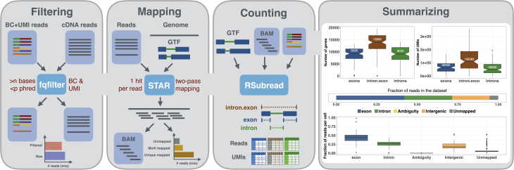
Findings: zUMIs is a pipeline that can handle both known and random BCs and also efficiently collapse UMIs, either just for exon mapping reads or for both exon and intron mapping reads. If BC annotation is missing, zUMIs can accurately detect intact cells from the distribution of sequencing reads. Another unique feature of zUMIs is the adaptive downsampling function that facilitates dealing with hugely varying library sizes but also allows the user to evaluate whether the library has been sequenced to saturation. To illustrate the utility of zUMIs, we analyzed a single-nucleus RNA-seq dataset and show that more than 35% of all reads map to introns. Also, we show that these intronic reads are informative about expression levels, significantly increasing the number of detected genes and improving the cluster resolution.

Conclusions: zUMIs flexibility makes if possible to accommodate data generated with any of the major scRNA-seq protocols that use BCs and UMIs and is the most feature-rich, fast, and user-friendly pipeline to process such scRNA-seq data.

Figure 1:

Schematic of the zUMIs pipeline. Each of the gray panels from left to right depicts a step of the zUMIs pipeline. First, fastq files are filtered according to user-defined bar code (BC) and unique molecular identifier (UMI) quality thresholds. Next, the remaining cDNA reads are mapped to the reference genome using STAR. Gene-wise read and UMI count tables are generated for exon, intron, and exon+intron overlapping reads. To obtain comparable library sizes, reads can be downsampled to a desired range during the counting step. In addition, zUMIs also generates data and plots for several quality measures, such as the number of detected genes/UMIs per BCe and distribution of reads into mapping feature categories.

Figure 2:

Comparison of different UMI collapsing methods. We compared Drop-seq-tools and UMI-tools with zUMIs using our HEK dataset (227 mio reads). (A) Run time to count exonic UMIs using zUMIs (hamming distance = 0), UMI-tools (”unique” mode) and Drop-seq-tools (edit distance = 0). (B) Box plots of correlation coefficients of gene-wise UMI counts of the same cell generated with different methods. UMI counts generated using zUMIs (quality filter “1 base under phred 17” or hamming distance = 1) were correlated to UMI counts generated using Drop-seq-tools (quality filter “1 base under phred 17” ) and UMI-tools (“directional adjacency” mode). (C) Comparison of the total number of UMIs per cell derived from different counting methods to “unfiltered” counts. (D) Violin plots of gene-wise dispersion estimates with different quality filtering and UMI collapsing methods.

Figure 3:

Utilities of zUMIs. Each of the panels shows the utilities of zUMIs pipeline. The plots from A–D show the results from the example HEK dataset used here. (A) The plot shows a density distribution of reads per BC. Cell BCs with reads right of the blue line are selected. (B) The plot shows the cumulative read distribution in the example HEK dataset where the BCs in light blue are the selected cells. (C)The bar plot shows the number of reads per selected cell BC with the red lines showing upper and lower median absolute deviation (MAD) cutoffs for adaptive downsampling. Here, the cells below the lower MAD have very low coverage and are discarded in downsampled count tables. (D) Cells were downsampled to six depths from 100,000 to 3,000,000 reads. For each sequencing depth, the genes detected per cell are shown. (E) Runtime for three datasets with 227, 500, and 1,000 million read-pairs. The runtime is divided in the main steps of the zUMIs pipeline as follows: filtering, mapping, counting, and summarizing. Each dataset was processed using 16 threads (“-p 16”).

Figure 4:

Contribution of intron reads to biological insights. We analyzed published single-nucleus RNA-seq data from mouse prefrontal cortex (PFC) and hippocampus [12] to assess the utility of counting intron in addition to exon reads. We processed the raw data with zUMIs to obtain expression tables with exon reads as well as exon+intron reads and then used the R-package Seurat [35, 36] to cluster cells. With exon counts, we identified 19 clusters (A), and with exon+intron counts we identified 27 clusters (B). Clusters are represented as t-SNE plots and colored according to the most frequent cell-type assignment in the original article [12]: glutamatergic neurons from the prefrontal cortex (exPFC), GABAergic interneurons (GABA), pyramidal neurons from the hippocampal CA region (CA), granule neurons from the hippocampal dentate gyrus region (DG), astrocytes (ASC), microglia (MG), oligodendrocytes (ODC), oligodendrocyte precursor cells (OPC), neuronal stem cells (NSC), smooth muscle cells (SMC) and endothelial cells (END). Different shades of those clusters indicate that multiple clusters had the same major cell type assigned. If we randomly sample counts from the intron data and add them to the exon counting, the noise reduces the number of clusters and the Seurat pipeline can only identify 9–11 clusters (E). The composition of each cluster based on exon+intron is detailed in panel (C), and cells that were not assigned a cell type in [12] are displayed as empty. The boxes mark the clusters that were not split when using exon data only. For example, cluster 7 from exon counting, which mainly consists of GABAergic neurons, was split into clusters 7, 24 (506, 66 cells) when using exon+intron counting. In (D), we show the numbers of genes that were differentially expressed (DE) (limma p-adj <0.05) between the clusters found only with exon+intron counts. The panel numbers represent the exon counting cluster numbers and the y-axis the exon+intron counting cluster number. The log2-fold changes corresponding to these contrasts are also used in (G). Among the genes that were additionally detected to be DE by exon+intron counting was the marker gene Il1rapl2 (limma p-adj = 10⁻⁵). In (F), we present a violin plot of the normalized counts for Il1rapl2 in cells of the GABAergic subclusters 7 and 24. Log2-fold changes calculated with exon+intron counts correlate well with exon counts (G). Note that for exon counting only, half as many genes could be evaluated as for exon+intron counting and thus only half of the exon+intron genes are depicted in (G). Large log₂ fold changes (LFCs) are found to be significant with both counting strategies (purple points are close to the bisecting line). We conducted simulations based on mean and dispersion measured using exon cluster 0 (1,616 cells, ∼90% exPFC). In (I) we show the expected true positive rate and the false discovery rate for a scenario comparing 300 vs 300 cells. Results for exon and exon+intron counting were stratified into five quantiles according to the mean expression of genes, where stratum 1 contains lowly expressed genes and stratum 5 the most highly expressed genes. The numbers of genes falling into each of the bins using exon+intron and exon counting are depicted in (H).

References

1. Sandberg R. Entering the era of single-cell transcriptomics in biology and medicine. Nat Methods. 2014;11(1):22–4. - PubMed
1. Zheng GXY, Terry JM, Belgrader P, et al. Massively parallel digital transcriptional profiling of single cells. Nat Commun. 2017;8:14049. - PMC - PubMed
1. Rosenberg AB, Roco CM, Muscat RA, et al. Single-cell profiling of the developing mouse brain and spinal cord with split-pool barcoding. Science. 2018;360(6385):176–82. - PMC - PubMed
1. Wagner A, Regev A, Yosef N. Revealing the vectors of cellular identity with single-cell genomics. Nat Biotechnol. 2016;34(11):1145–60. - PMC - PubMed
1. Regev A, Teichmann SA, Lander ES, et al. The Human Cell Atlas. Elife, 2017; 6. - PMC - PubMed
Publication types