Flexible Sensorimotor Computations through Rapid Reconfiguration of Cortical Dynamics

Abstract

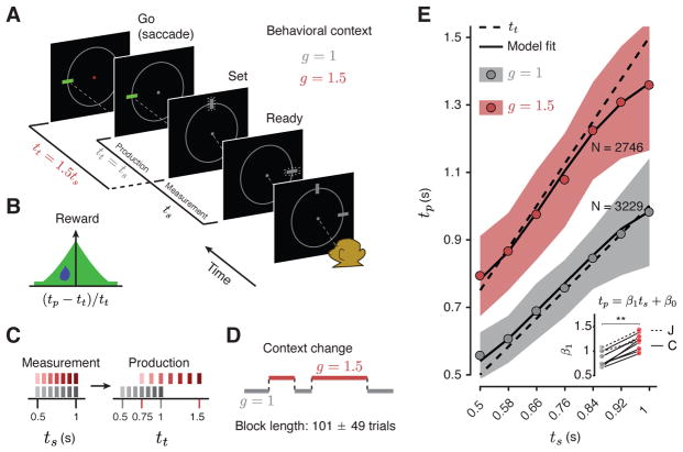
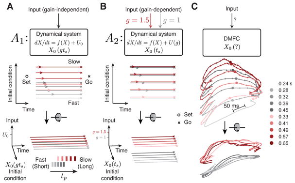
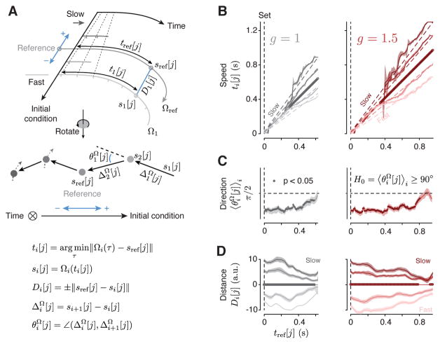
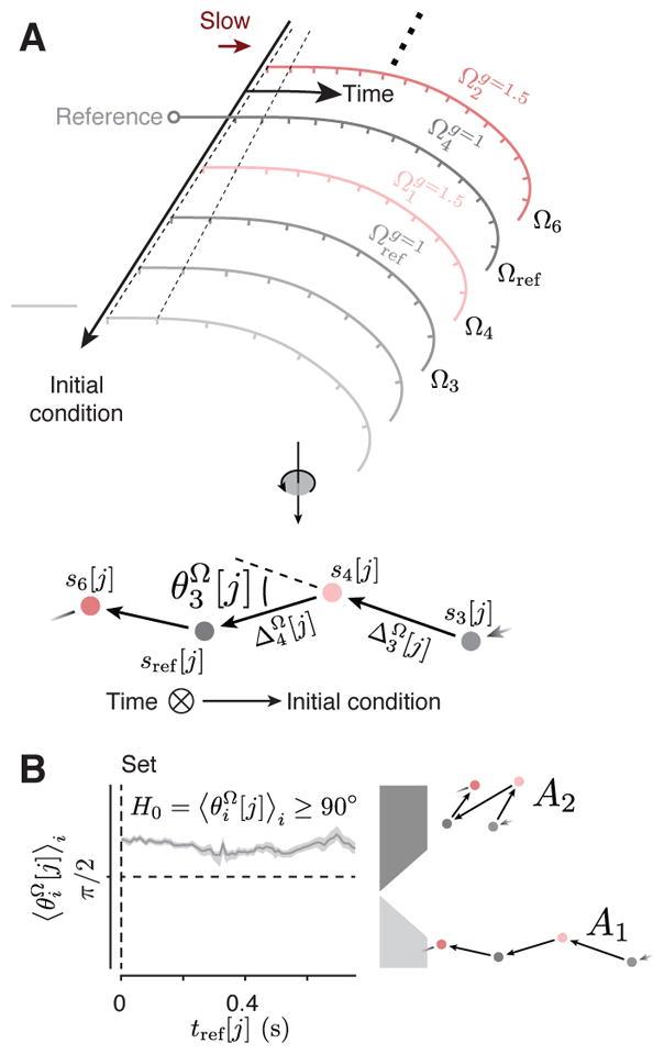
Neural mechanisms that support flexible sensorimotor computations are not well understood. In a dynamical system whose state is determined by interactions among neurons, computations can be rapidly reconfigured by controlling the system's inputs and initial conditions. To investigate whether the brain employs such control mechanisms, we recorded from the dorsomedial frontal cortex of monkeys trained to measure and produce time intervals in two sensorimotor contexts. The geometry of neural trajectories during the production epoch was consistent with a mechanism wherein the measured interval and sensorimotor context exerted control over cortical dynamics by adjusting the system's initial condition and input, respectively. These adjustments, in turn, set the speed at which activity evolved in the production epoch, allowing the animal to flexibly produce different time intervals. These results provide evidence that the language of dynamical systems can be used to parsimoniously link brain activity to sensorimotor computations.

Keywords: Dynamical Systems; cognitive flexibility; electrophysiology; frontal cortex; motor planning; population coding; recurrent neural networks; sensorimotor coordination; timing.

Figure 1. The RSG task and behavior

(A) RSG task. On each trial, three rectangular stimuli associated with “Ready,” “Set,” and “Go” events were shown on the screen arranged in a semi-circle. Following fixation, Ready and Set cues were extinguished. After a random delay, first Ready and then Set stimuli were flashed (small lines around the rectangles signify flashed stimuli). The time interval between Ready and Set demarcated a sample interval, t_s. The monkey’s task was to generate a saccade (“Go”) to a visual target such that the interval between Set and Go (produced interval, t_p) was equal to a target interval, t_t, equal to t_s multiplied by a gain factor, g (t_t = gt_s). The animal had to perform the task in two behavioral contexts, one in which t_t was equal to t_s (g = 1 context), and one in which t_t was 50% longer than t_s (g = 1.5 context). The context was cued throughout the trial by the color of fixation and the position of a context stimulus (small white square below the fixation). (B) Reward. Animals received juice reward when the error between t_p and t_t was small, and the reward magnitude decreased with the size of error (see Methods for details). On rewarded trials, the saccadic target turned green (panel A). (C) Sample and target intervals. For both contexts, t_s was drawn from a discrete uniform distribution with seven values equally spaced from 0.5 to 1 sec (left). The values of t_s were chosen such that the corresponding values of t_t across the two contexts were different but partially overlapping (right). (D) Context blocks. The context changed across blocks of trials. The number of trials in a block was varied pseudorandomly (mean and std shown). (E) Behavior. t_p as a function of t_s for each context across both monkeys and all recording sessions (behavior of each animal is shown separately in Figure S1). Circles indicate mean t_p across all sessions, shaded regions indicate +/− one standard deviation from the mean, dashed lines indicate t_t, and solid lines are the fits of a Bayesian observer model to behavior. Inset: Slope of the regression line (β₁) relating t_p to t_s in the two contexts. Regression slopes were larger in the g = 1.5 context, with a significant interaction between t_s and g (p < 0.0001) for all sessions (see text; ** indicates p < 0.002 for signed-rank test). Regression intercepts (β₀) were also larger for the g = 1.5 context (0.14 vs. 0.18 sec, p = 0.04). In all panels, different shades of gray and red are associated with g =1 and g = 1.5, respectively. See Figure S1 for individual animals.

Figure 2. Neural responses in dorsomedial frontal cortex during the RSG task

(A) Example neurons. Firing rates of 5 example units during the various phases of the task aligned to Ready (left column), Set (middle) and Go (right). Responses aligned to Ready and Set were sorted by t_s. Responses aligned to Go were sorted into 5 bins, each with the same number of trials, ordered by t_p. Gray and red lines correspond to activity during the g =1 and g = 1.5 contexts, respectively, with darker lines corresponding to longer intervals. (B) Population activity during Ready-Set. Visualization of population activity in the Ready-Set epoch sorted by t_s. The “gain axis” corresponds to the axis along which responses were maximally separated with respect to context at the time of Set. The other two dimensions (“PC1 and PC2”) correspond to the first two principal components of the data after removing the context dimension. Inset: fraction of variance explained by first 25 principal components. Dashed line indicates 100%. (C) Population activity during Set-Go. Visualization of population activity in the Set-Go epoch sorted into 5 bins, each with the same number of trials, ordered by t_p. Top: Activity plotted in 2 dimensions spanned by PC1 and the dimension of maximum variance with respect to t_p within each context (“Interval axis”). Bottom: Same as Top rotated 90 degree (circular arrow) to visualize activity in the plane spanned by the context axis (“Gain axis”) and PC1. For plotting purposes, PCs were orthogonalized with respect to the interval and gain axes. Squares, circles, and crosses in the state space plots represent Ready, Set, and Go, respectively. Percentage variance explained by interval and gain are shown numerically near the corresponding axes. See methods for the calculation of percent variance explained by interval and gain. See Figure S2 for individual animals and Figure S11 for different recording sites.

Figure 3. Dynamical systems predictions for the RSG task

(A,B) Schematic illustrations of two hypothetical dynamical systems solutions to RSG across contexts through manipulation of initial conditions or external inputs. (A) The first solution (A₁). Top: In A₁, the initial condition (X₀) depends on the target interval t_t = gt_s (g, gain, t_s, sample interval), and the system is driven by a gain-independent input (U₀). Middle: state trajectory between Set and Go in the plane spanned by initial condition and time axes. After Set (open circles), activity evolves towards an action-triggering state (crosses) with a speed (colored arrows) fully determined by position along the initial condition axis (ordinate). Activity across contexts is organized according to t_t = gt_s. Bottom: same trajectories, rotated to show an oblique view. Trajectories are separated only along the initial condition axis across both contexts such that trajectory structure reflects t_t explicitly. There is no separation along the Input axis. (B) The second solution (A₂). Top: In A₂, X₀ depends on t_s within contexts, but the system is driven by a tonic gain-dependent input (U (g) ; red and gray arrow for the two gains). Middle: state trajectory between Set and Go in the plane spanned by initial condition and time axes. Because initial condition encodes t_s and not t_t, in this plane, trajectories associated with the same t_s but different gains appear overlapping. Bottom: oblique view. A context-dependent external input creates two sets of neural trajectories in the state space for the two contexts in the Set-Go epoch. This input controls speed in conjunction with initial conditions, generating a structure which reflects t_s and g explicitly, but not t_t. In both A₁ and A₂, responses would be initiated when activity projected onto the time axis reaches a threshold. (C) DMFC data. Top: unknown mechanism of RSG control in DMFC. Middle, bottom: 3-dimensional projection of DMFC activity in the Set-Go epoch (from Figure 2C). Middle: qualitative assessment indicated that neural trajectories within each context for different t_p bins were associated with different initial conditions and remained separate and ordered through the response. Bottom: Across the two contexts, neural trajectories formed two separated sets of neural trajectories without altering their relative organization as a function of t_p. Both of these features were consistent with A₂. Filled circles depict states along each trajectory at a constant fraction of the trajectory length, illustrating speed differences across trajectories (circles are closer for the longer intervals associated with slower speed).

Figure 4. Kinematic analysis of neural trajectories (KiNeT)

(A) Illustration of KiNeT. Top: a collection of trajectories originate from Set, organized by initial condition, and terminate at Go. Tick marks on the trajectories indicate unit time. Darker trajectories evolve at a lower speed as demonstrated by the distance between tick marks and the dashed line connecting tick marks. KiNeT quantifies the position of trajectories and the speed with which states evolve along them relative to a reference trajectory (middle trajectory, Ω_ref). To do so, it finds a collection of states {s_i[j]}_j on each Ω_i that are closest to Ω_ref through time. Trajectories which evolve at a slower speed require more time to reach those states leading to larger values of t_i[j]. KiNet quantifies relative position by a distance measure, D_i[j] (distance between Ω_i and Ω_ref at t_i[j]) that is signed (blue arrows) and is considered positive when Ω_i corresponds to larger values of t_p (slower trajectories). Middle: trajectories rotated such that the time axis is normal to the plane of illustration, denoted by a circle with an inscribed cross. Filled circles represent the states {s_i[j]}_j aligned to s_ref[j] for a particular j. Vectors ${\mathrm{\Delta }}_i^{\mathrm{\Omega }}[j]$ connect states on trajectories of shorter to longer t_p. Angles ${\theta }_i^{\mathrm{\Omega }}[j]$ between successive ${\mathrm{\Delta }}_i^{\mathrm{\Omega }}[j]$ provide a measure of t_p-related structure. Bottom: equations defining the relevant variables. (B) Speed of neural trajectories compared to Ω_ref computed for each context separately. Shortly after Set, all trajectories evolved with similar speed (unity slope). Afterwards, Ω_i associated with shorter t_s evolved faster than Ω_ref as indicated by a slope of less than unity (i.e., {t_i [j]}_j smaller than {t_ref [j]}_j), and Ω_i associated with longer t_s evolved slower than Ω_ref. Filled circles on the unity line indicate j values for which {t_i [j]}_j was significantly correlated with i (bootstrap test, r > 0, p < 0.05, n = 100). (C) Relative position of adjacent neural trajectories computed for each context separately. ${\langle {\theta }_i^{\mathrm{\Omega }}[j]\rangle }_i$ (angle brackets signify average across trajectories) were significantly smaller than 90 degrees (filled circle) for the majority of the Set-Go epoch (bootstrap test, ${\langle {\theta }_i^{\mathrm{\Omega }}[j]\rangle }_i<90$, p < 0.05, n = 100) indicating that ${\mathrm{\Delta }}_i^{\mathrm{\Omega }}[j]$ were similar across Ω_i. (D) Distance of neural trajectories to Ω_ref computed for each context separately. Distance measures (D_i[j]) indicated that {Ω_i}_i had the same ordering as the corresponding t_p values. The magnitude of D_i[j] decreased with time indicating that trajectories coalesce as they get closer to the time of Go. When trajectories coalesce, small deviations in their relative position due to variability in firing rate estimates may cause trajectories to appear disorganized. This is consistent with the observation that ${\langle {\theta }_i^{\mathrm{\Omega }}[j]\rangle }_i$ were closer to 90 degrees near the time of Go (panel C). Significance was tested using bootstrap samples for each j (p < 0.05, n = 100). See Figure S5 for individual animals and Figure S11 for different recording sites.

Figure 5. Neural trajectories across contexts do not form a single structure reflecting

t_p. (A) A schematic illustrating neural trajectories across the two contexts after Set. Top: The expected geometrical structure under A₁. Neural trajectories for the gain of 1 (gray) and 1.5 (red) are organized along a single initial condition axis and ordered with respect to t_p. Tick marks indicate unit time. Bottom: A rotation of the top showing neural trajectories with the time axis normal to the plane of illustration. If the neural trajectories were organized as such, then the angle between vectors connecting nearby points (e.g., ${\theta }_3^{\mathrm{\Omega }}[j]$) would be less than 90 (A₁, Figure 3A). (B) Left: orientation of vectors connecting adjacent neural trajectories combined across the two contexts. Right: possible geometrical structures A₁ (bottom), and A₂ (top). ${\langle {\theta }_i^{\mathrm{\Omega }}[j]\rangle }_i$ was larger than 90 degrees for all j in the Set-Go interval, consistent with A₂. Shaded regions represent 90% bootstrap confidence intervals. See Figure S6 for individual animals and Figure S11 for different recording sites.

Figure 6. Neural trajectories comprise distinct but similar structures across gains

(A) A schematic showing the organization of neural trajectories in a subspace spanned by Input, Initial condition and Time if context were controlled by tonic external input. If DMFC were to receive a gain-dependent input, we would expect neural trajectories from Set to Go to be separated along an input subspace, generating two similar but separated t_p-related structures for each context (A₂, Figure 3B). We verified this geometrical structure by excluding alternative structures (interdictory circles indicate rejected alternatives). (B) An illustration of neural trajectories for g =1 (gray filled circle) and g = 1.5 (red filled circle) with the time axis normal to the plane of illustration. Gray and red arrows show vectors connecting nearby points in each context independently (Δ^Ω,g=1.5 and Δ^Ω,g=1). When the neural trajectories associated with the two gains are structured similarly, these vectors are aligned and the angle between them (θ^g) is less than 90 deg. We used KiNeT to test this possibility (see Methods). (C) Left: Schematic illustrating a condition in which the time axis for trajectories in the two contexts (gray and red) are not aligned. Right: ${\left\{t_{\text{ref}}^{g=1}[j]\right\}}_j$ increased monotonically with ${\left\{t_{\text{ref}}^{g=1.5}[j]\right\}}_j$ indicating that the time axes across contexts were aligned. Values of ${\left\{t_{\text{ref}}^{g=1.5}[j]\right\}}_j$ above the unity line indicate that activity evolved at a slower speed in the g = 1.5 context. The dashed gray line represents unity and the dashed red line represent expected values for ${\left\{t_{\text{ref}}^{g=1.5}[j]\right\}}_j$ if speeds were scaled perfectly by a factor of 1.5. (D) Left: Schematic illustrating an example configuration in which ${\left\{{\mathrm{\Omega }}_i^{g=1}\right\}}_i$ and ${\left\{{\mathrm{\Omega }}_i^{g=1.5}\right\}}_i$ establish dissimilar t_p-related structures. Right: ${\langle {\theta }_i^{\mathrm{\Omega }}[j]\rangle }_i$ was significantly less than 90 degrees for all j indicating that the t_p-structure was similar across the two contexts. (E). Left: Schematic illustrating a condition in which ${\left\{{\mathrm{\Omega }}_i^{g=1}\right\}}_i$ and ${\left\{{\mathrm{\Omega }}_i^{g=1.5}\right\}}_i$ are overlapping. Right: The minimum distance D^g across contexts (black line) was substantially larger than that found between subsets of trajectories within contexts (red and gray lines, see Methods) indicating the two sets of trajectories were not overlapping. (F) Left: Schematic illustrating a condition in which ${\left\{{\mathrm{\Omega }}_i^{g=1}\right\}}_i$ and ${\left\{{\mathrm{\Omega }}_i^{g=1.5}\right\}}_i$ are separated along the same direction that neural trajectories within each context were separated. Right: The vector associated with the minimum distance between the two manifolds (Δ^g[j]) was orthogonal to the vector connecting nearby states for both $g=1(\text{gray},{\langle {\mathrm{\Delta }}_i^{\mathrm{\Omega },g=1}[j]\rangle }_i)$ and $g=1.5(\text{red},{\langle {\mathrm{\Delta }}_i^{\mathrm{\Omega },g=1.5}[j]\rangle }_i)$. In (C–E), shaded regions represent 90% bootstrap confidence intervals, and circles represent statistical significance (p < 0.05, bootstrap test, n = 100). See Figure S7 for individual animals and Figure S11 for different recording sites.

Figure 7

Relating neural variability to behavioral variability. (A). Schematic showing states (filled circles) along three neural trajectories (gray lines) between Set (circle) and Go (cross) associated with three different t_s values. The light and dark stars depict two neural states that are deviated from the average neural trajectory (the middle trajectory). The light star corresponds to trials in which t_p was shorter than median $t_p(s_i^{\text{short}}[j])$), and the dark star, to trials in which t_p was longer than median ( $s_i^{\text{long}}[j]$). $s_i^{\text{short}}[j]$ is deviated from the average trajectory in the direction of shorter t_s (toward s_{i − 1}[j] by vector ò^Ω) and in the direction of the Go state (toward s_i[j+1] by vector ò^t). The opposite is true for $s_i^{\text{long}}[j]$. (B) Prediction 1 (P₁): deviations ò^Ω off of one trajectory toward a trajectory associated with longer t_s should lead to longer t_p, and vice versa. The dashed arrow represents ${\mathrm{\Delta }}_i^p[j]$, the vector pointing from $s_i^{\text{short}}[j]$ to $s_i^{\text{long}}[j]$, and the blue arrow represents ${\mathrm{\Delta }}_i^{\mathrm{\Omega }}[j]$, the vector pointing from s_{i − 1}[j] to s_{i +1}[j]. P₁ is satisfied if the angle between these vectors, denoted by ${\theta }_i^{p,\mathrm{\Omega }}[j]$, is acute. (C) Prediction 2 (P₂): deviations ò^t along trajectories should influence the time it takes for activity to reach the Go state and should therefore influence t_p. The green arrow represents ${\mathrm{\Delta }}_i^{\mathrm{\Omega }}[j]$, the vector that connects s_i [j − 1] to s_i [j + 1]. If P₂ is correct, the angle ${\theta }_i^{p,t}[j]$ between ${\mathrm{\Delta }}_i^p[j]$ and ${\mathrm{\Delta }}_i^t[j]$ should be obtuse. (D,E) Testing P₁ and P₂ for the g = 1 (D) and g = 1.5 (E) contexts. Consistent with P₁, average ${\theta }_i^{p,\mathrm{\Omega }}[j]({\langle {\theta }_i^{p,\mathrm{\Omega }}[j]\rangle }_i,\text{blue})$ was less than 90 deg from Set to Go indicating that t_p was longer (shorter) when neural states deviated toward a trajectory associated with a longer (shorter) t_s. Consistent with P₂, ${\langle {\theta }_i^{p,t}[j]\rangle }_i$ (green) was greater than 90 deg, indicating that t_p was longer (shorter) when speed along the neural trajectory was slower (faster). The average angle between ${\mathrm{\Delta }}_i^{\mathrm{\Omega }}[j]$ and ${\mathrm{\Delta }}_i^t[j]{\langle {\theta }_i^{\mathrm{\Omega },t}[j]\rangle }_i$ (yellow) was not significantly different than expected by chance (90 deg) for most time points. We determined when (at what j) an angle was significantly different from 90 deg (p < 0.05) by comparing angles to the corresponding null distribution derived from 100 random shuffles with respect to t_p. Angles that were significantly different from 90 deg are shown by darker circles. See Figure S8 for individual animals and Figure S11 for different recording sites.

Figure 8. RNNs with tonic but not transient input captured the structure of activity in DMFC

(A) Schematic illustration of the RNNs. The networks receive brief Ready and Set pulses separated in time by t_s. Additionally, each network is provided with a context-dependent “input” which either terminates prior to Ready (“Transient input,” top), or persists throughout the trial (“Tonic input,” bottom). All networks were trained so that the output (z) would generate a ramp after Set that would reach a threshold (dashed line) at the context-dependent t_t. (B) Top: state-space projections of tonic-input RNN activity in the Set-Go epoch. The axes for 3D projections were identified using the same method as in Figure 2C. (C) Same as panel B for the transient-input RNN. (D) Analysis of direction in the tonic-input RNN with the same format as Figure 5B. ${\langle {\theta }_i^{\mathrm{\Omega }}[j]\rangle }_i$ was larger than 90 deg for the entire the Set-Go epoch. This indicates that the tonic network forms two separate context-specific sets of isomorphic neural trajectories (inset). (E) Same as panel D for the transient-input network. ${\langle {\theta }_i^{\mathrm{\Omega }}[j]\rangle }_i$ was consistently less than 90 deg consistent with a geometry in which neural trajectories are organized with respect to t_p regardless of the gain context (inset). (F,G) Trajectory separation (D^g) across contexts for the tonic-input (F) and transient-input (G) networks with the same format as Figure 6E. D^g was substantially larger through the Set-Go epoch in the tonic-input network (F). In (D–G), shaded regions represent 90% bootstrap confidence intervals, and circles represent statistical significance (p < 0.05, bootstrap test, n = 100). See Figure S10 for a more detailed analysis of RNN results.

References

1. Acerbi L, Wolpert DM, Vijayakumar S. Internal representations of temporal statistics and feedback calibrate motor-sensory interval timing. PLoS computational biology. 2012;8(11):e1002771. doi: 10.1371/journal.pcbi.1002771. - DOI - PMC - PubMed
1. Afshar A, Santhanam G, Yu BM, et al. Single-trial neural correlates of arm movement preparation. Neuron. 2011;71(3):555–564. doi: 10.1016/j.neuron.2011.05.047. - DOI - PMC - PubMed
1. Akkal D, Dum RP, Strick PL. Supplementary motor area and presupplementary motor area: targets of basal ganglia and cerebellar output. The Journal of neuroscience: the official journal of the Society for Neuroscience. 2007;27(40):10659–10673. doi: 10.1523/JNEUROSCI.3134-07.2007. - DOI - PMC - PubMed
1. Bates JF, Goldman-Rakic PS. Prefrontal connections of medial motor areas in the rhesus monkey. The Journal of comparative neurology. 1993;336(2):211–228. doi: 10.1002/cne.903360205. - DOI - PubMed
1. Brass M, von Cramon DY. The role of the frontal cortex in task preparation. Cerebral cortex. 2002;12(9):908–914. doi: 10.1093/cercor/12.9.908. - DOI - PubMed
Publication types
LinkOut - more resources