Size-strain separation in diffraction line profile analysis

Abstract

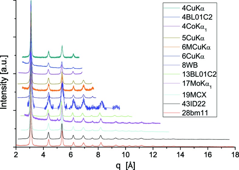
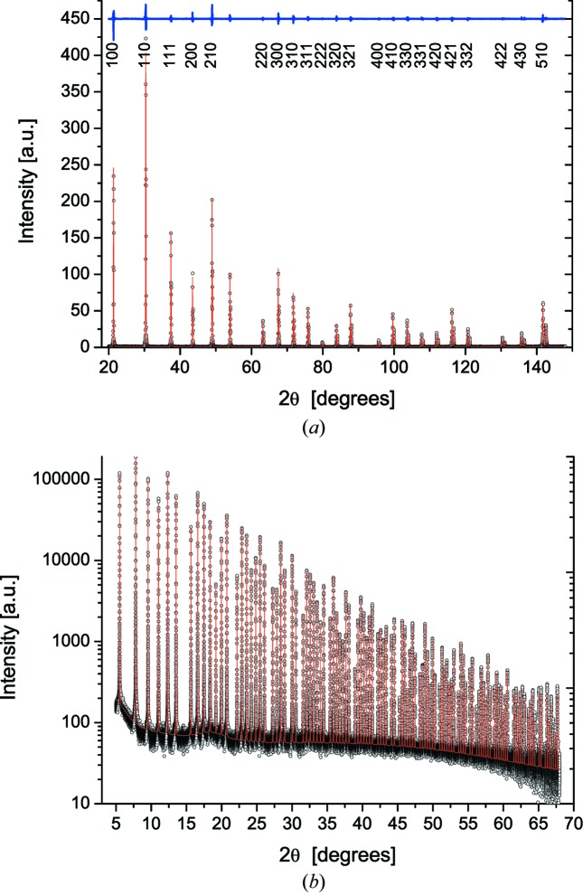
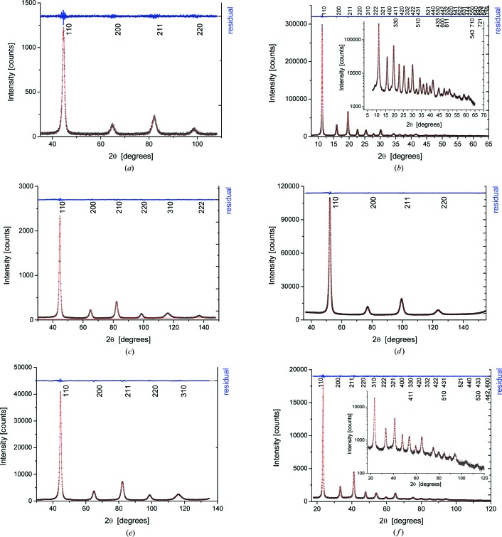
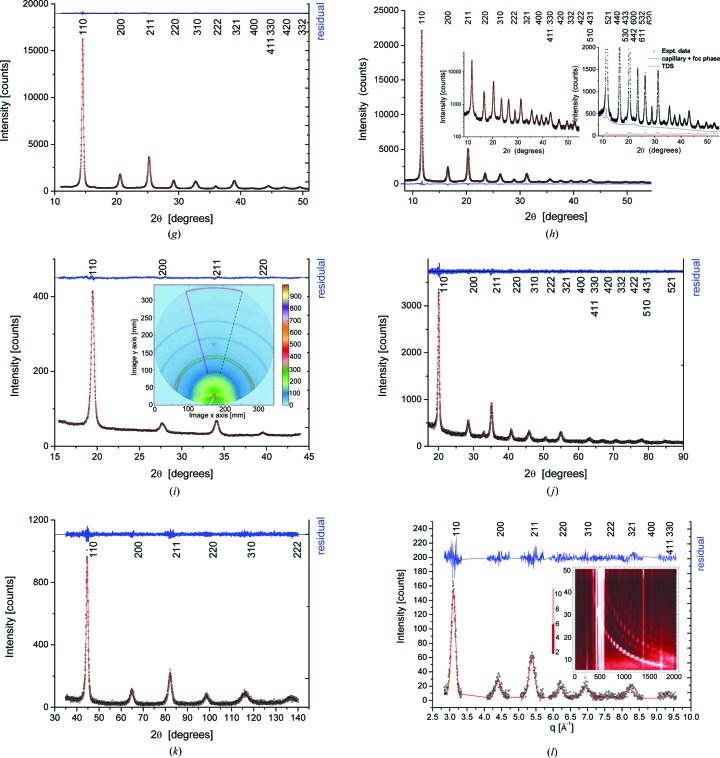
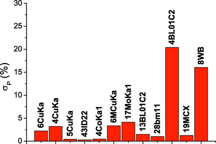
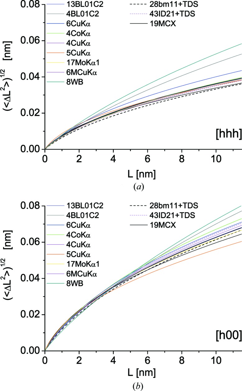
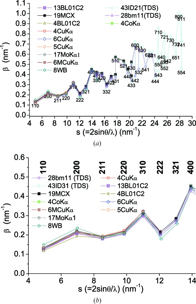
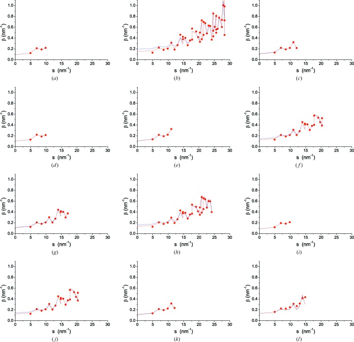
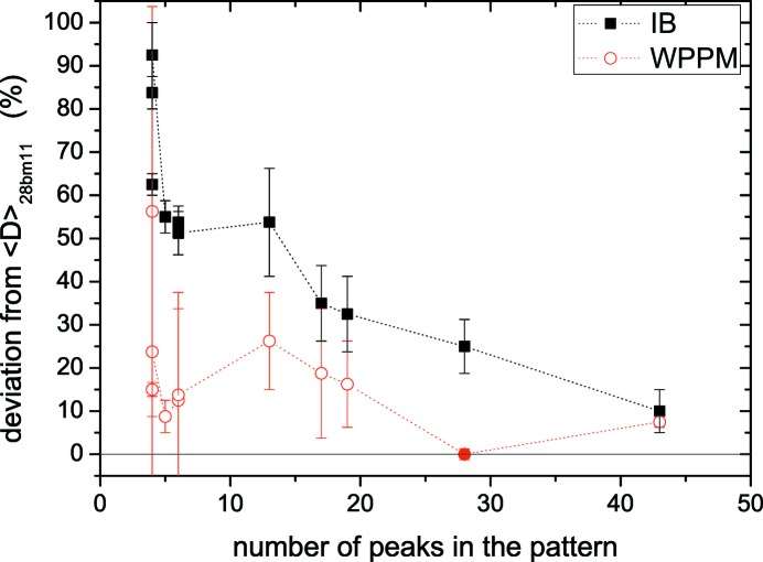
Separation of size and strain effects on diffraction line profiles has been studied in a round robin involving laboratory instruments and synchrotron radiation beamlines operating with different radiation, optics, detectors and experimental configurations. The studied sample, an extensively ball milled iron alloy powder, provides an ideal test case, as domain size broadening and strain broadening are of comparable size. The high energy available at some synchrotron radiation beamlines provides the best conditions for an accurate analysis of the line profiles, as the size-strain separation clearly benefits from a large number of Bragg peaks in the pattern; high counts, reliable intensity values in low-absorption conditions, smooth background and data collection at different temperatures also support the possibility to include diffuse scattering in the analysis, for the most reliable assessment of the line broadening effect. However, results of the round robin show that good quality information on domain size distribution and microstrain can also be obtained using standard laboratory equipment, even when patterns include relatively few Bragg peaks, provided that the data are of good quality in terms of high counts and low and smooth background.

Keywords: crystalline domain size; line profile analysis; microstrain; powder diffraction.

Figure 1

Synoptic view of all data collected for this study. All patterns were collected at room temperature [with the exception of 11bm, where data (not shown here) are also available at 100 and 200 K]. To allow for a direct comparison, all patterns are shown as intensity in arbitrary units versus q, and are scaled upward according to the extension in q space.

Figure 2

Whole pattern fitting of LaB₆ standard data, using pV profile functions. (a) Cu Kα_1,2 data (6CuKα) with indication of residual (above, difference between experimental and fitting profile) and Miller indices. (b) 43ID22 with 31 keV radiation: and modelling using pV profile functions for 119 peaks of LaB₆ (NIST SRM660b). Note the linear scale in (a) versus the logarithmic scale in (b). See supporting information for results for all instruments in this study.

Figure 3

(a) Parameterization of IP (FWHM and η) from the data in Fig. 2 ▸(a). Refined coefficients for the 6CuKα laboratory instrument (Fig. 2 ▸ a) are W = 5.906369 × 10⁻³, V = −2.502974 × 10⁻³, U = 3.712228 × 10⁻³, a = 3.107787 × 10⁻¹, b = 6.175673 × 10⁻³, c = 0. The lower line is the tanθ polynomial correcting aberrations on peak position [equation (4)] (Wilson, 1963 ▸), with refined parameters a ₋₁ = −5.978103 × 10⁻⁴, a ₀ = 1.437456 × 10⁻², a ₁ = −9.797414 × 10⁻³, a ₂ = 0, a ₃ = 2.635631 × 10⁻⁴. (b) The same analysis is made for the pattern in Fig. 2 ▸(b), 43ID22 with 31 keV radiation, showing a much narrower IP than in (a), and nearly negligible peak position correction; the inset shows data with a ×10 expansion of left ordinate axis. For most instruments η varies linearly with θ, as in the cases in this figure, or is even constant as for SR data. See supporting information for results for all instruments in this study.

Figure 4

Experimental data (circular data points), modelling (line) and their difference (residual, upper line). (a) 4CuKα; (b) 43ID22, with detail in log scale in the inset; (c) 6CuKα; (d) 4CoKα₁; (e) 5CuKα; (f) 19MCX 15 keV; (g) 13BL01C2 24 keV; (h) 28bm11 30 keV; (i) 4BL01C2 18 keV, with detail of the imaging plate reading in the inset; (j) 17MoKα₁ (the unindexed peak at 33° is a spurious effect of scattering from the glass capillary); (k) 6MCuKα; (l) 8WB, with the density plot of angle versus energy shown in the inset. Miller indices are shown in each plot.

Figure 4

Experimental data (circular data points), modelling (line) and their difference (residual, upper line). (a) 4CuKα; (b) 43ID22, with detail in log scale in the inset; (c) 6CuKα; (d) 4CoKα₁; (e) 5CuKα; (f) 19MCX 15 keV; (g) 13BL01C2 24 keV; (h) 28bm11 30 keV; (i) 4BL01C2 18 keV, with detail of the imaging plate reading in the inset; (j) 17MoKα₁ (the unindexed peak at 33° is a spurious effect of scattering from the glass capillary); (k) 6MCuKα; (l) 8WB, with the density plot of angle versus energy shown in the inset. Miller indices are shown in each plot.

Figure 5

Comparison of counting statistics of the different data sets, expressed as standard deviation of the intensity distribution (Klug & Alexander, 1974 ▸), , where N _T and N _B are, respectively, total and background intensity.

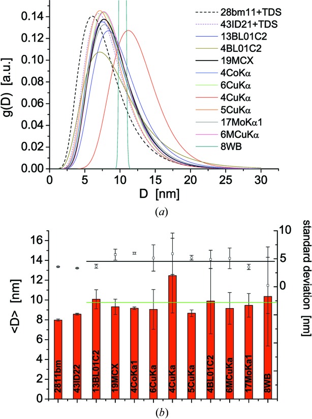
Figure 6

(a) Lognormal size distribution, g(D), from WPPM of all patterns in this study; (b) mean size, 〈D〉, and standard deviation of the distribution. The green line in (b) is the weighted average of all mean sizes (except 28bm11 and 43ID22, where WPPM included the TDS contribution: see text for details).

Figure 7

Warren plots for all samples in the study. Trend of the variance of the atomic displacement distribution as a function of the distance L between pairs of atoms along the two directions, (a) [hhh] and (b) [h00], corresponding to soft and stiff elastic response in ferritic iron, respectively.

Figure 8

(a) Integral breadth, β(s), as a function of s = 2sinθ/λ, for all data in the present study. A detail of the low-s region is shown in (b).

Figure 9

Results of the mWH analysis. Data points (circles) from equation (13); fit by least squares using equation (16) without (blue line) or with (red line) weights (relative integrated intensity). With few data points the two trends, with and without weights, overlap nearly identically. (a) 4CuKα; (b) 43ID22; (c) 6CuKα; (d) 4CoKα₁; (e) 5CuKα; (f) 19MCX; (g) 13BL01C2; (h) 28bm11; (i) 4BL01C2; (j) 17MoKα₁; (k) 6MCuKα; (l) 8WB.

Figure 10

Deviation of mean domain size from the reference WPPM value for 28bm11 data, (〈D〉 − 〈D〉_28bm11)/〈D〉_28bm11, as a function of the number of peaks in the pattern. The mean size is calculated by the integral breadth (mWH) method (squares) and by WPPM (open circles; filled circle for the reference data).

References

1. Adler, T. & Houska, C. R. (1979). J. Appl. Phys. 50, 3282–3287.
1. Armstrong, N., Cline, J. P., Ritter, J. & Bonevich, J. (2005). Acta Cryst. A61, C79.
1. Balzar, D., Audebrand, N., Daymond, M. R., Fitch, A., Hewat, A., Langford, J. I., Le Bail, A., Louër, D., Masson, O., McCowan, C. N., Popa, N. C., Stephens, P. W. & Toby, B. H. (2004). J. Appl. Cryst. 37, 911–924.
1. Bertaut, E. F. (1950). Acta Cryst. 3, 14–18.
1. Beyerlein, K. R., Leoni, M. & Scardi, P. (2012). Acta Cryst. A68, 382–392. - PubMed