Spatial relationship between bone formation and mechanical stimulus within cortical bone: Combining 3D fluorochrome mapping and poroelastic finite element modelling

Abstract

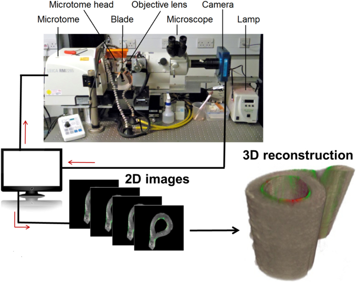
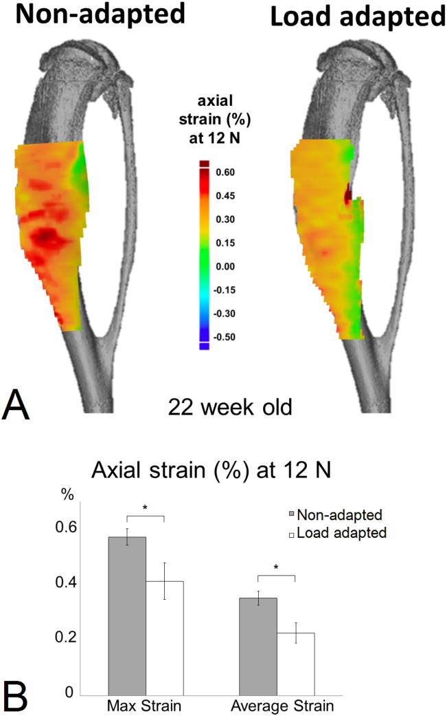
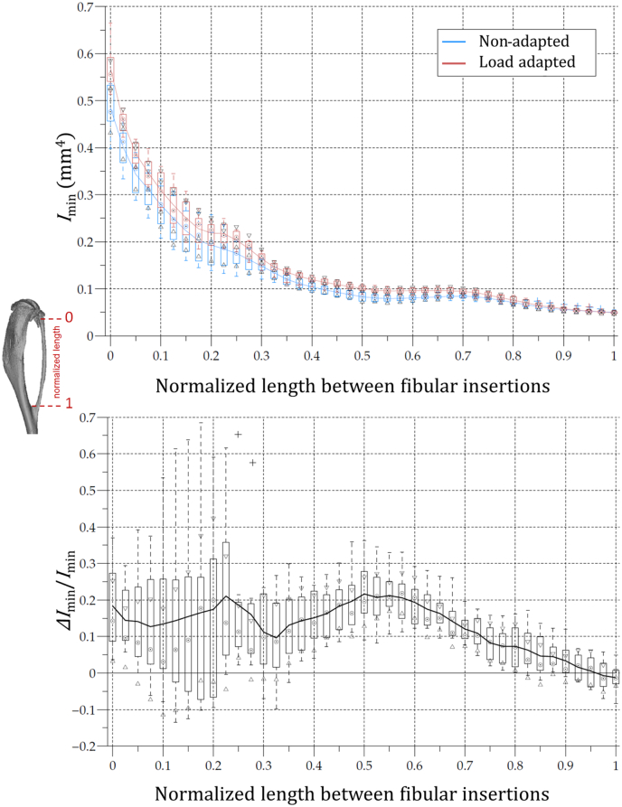
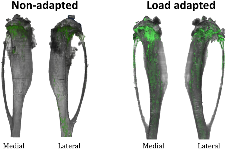
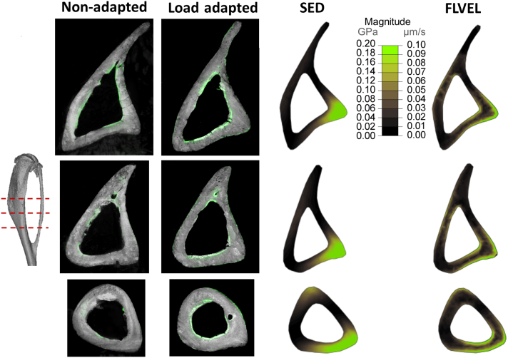
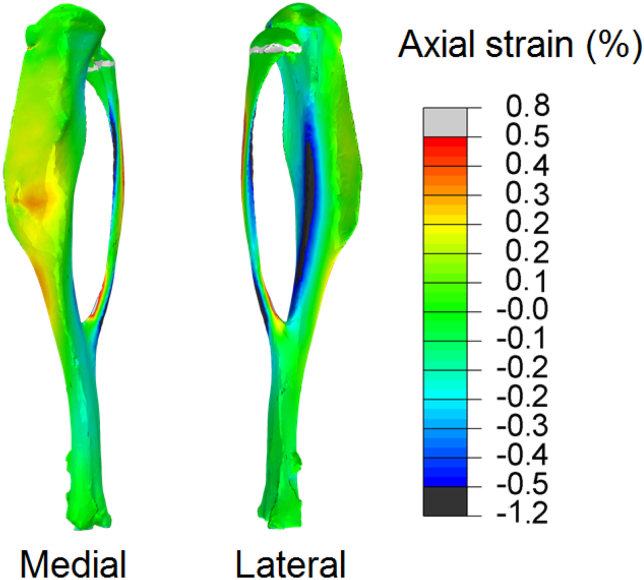
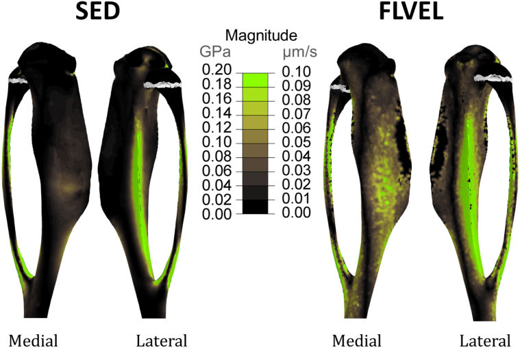
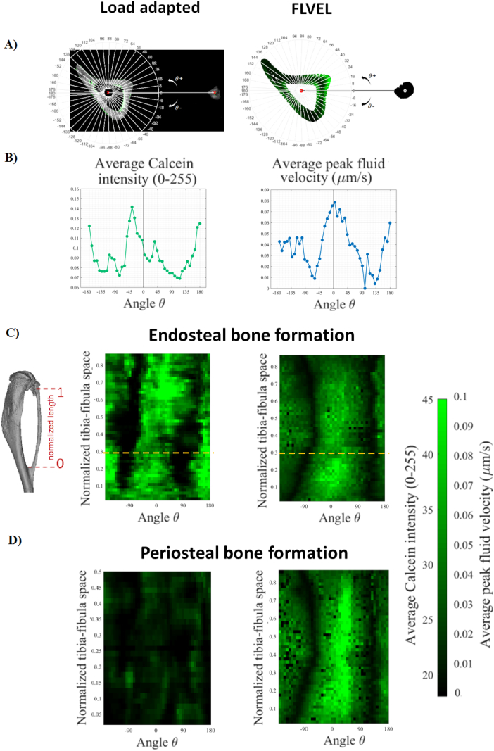
Bone is a dynamic tissue and adapts its architecture in response to biological and mechanical factors. Here we investigate how cortical bone formation is spatially controlled by the local mechanical environment in the murine tibia axial loading model (C57BL/6). We obtained 3D locations of new bone formation by performing 'slice and view' 3D fluorochrome mapping of the entire bone and compared these sites with the regions of high fluid velocity or strain energy density estimated using a finite element model, validated with ex-vivo bone surface strain map acquired ex-vivo using digital image correlation. For the comparison, 2D maps of the average bone formation and peak mechanical stimulus on the tibial endosteal and periosteal surface across the entire cortical surface were created. Results showed that bone formed on the periosteal and endosteal surface in regions of high fluid flow. Peak strain energy density predicted only the formation of bone periosteally. Understanding how the mechanical stimuli spatially relates with regions of cortical bone formation in response to loading will eventually guide loading regime therapies to maintain or restore bone mass in specific sites in skeletal pathologies.

Keywords: 3D fluorochrome mapping; Bone adaptation; Cortical bone; Mouse; Tibia.

Fig. 1

Schematic of the automatic imaging acquisition and bone reconstruction used during 3D fluorochrome mapping. The histocutter is a combination of the microtome for automatic cutting and a fluorescence microscope for image acquisition. The fluorescence microscope has UV, green, and red emission filters. A grey scale CCD camera positioned behind the fluorescence microscope captures the fluorescence light emitted by the sample. The distance between the camera and the exposed surface is fixed to ensure a constant focus through a series of slicing and imaging process. An in-house custom written code synchronizes the microtome action, filter wheels, shutters, and the camera operation for capturing the imaging that is then sent to a hard disk for storage. In this study, we used a 3.3-x objective with a 1.591 μm in-plane resolution and a field of view of 4.585 mm. We imaged the bone sample using an ultraviolet (UV) excitation filter (excitation 365, emission 450; Nikon), the calcein fluorescence using a green filter (excitation 480, emission 535; Nikon) and alizarin red using a red filter (excitation 560, emission 645; Nikon). About 3000 sections were imaged at a distance of 5 um for each bone, thus collecting 6000 images. (For interpretation of the references to colour in this figure legend, the reader is referred to the web version of this article.)

Fig. 2

(A) The strain map on the bone surface at 12 N of load assessed with a DIC system on a representative control and loaded 22 week-old mouse tibia (images for the load adapted tibia are reflected to allow a direct comparison with those of the control, non-loaded tibia). (B) Peak and average strain measured on the bone surface of 5 control and 5 loaded samples at 12 N. (^⁎ indicates p < 0.001).

Fig. 3

Boxplot representation of the 22 w.o. mouse tibial second moment of area about the minor axis (I_min) of the control (blue) and loaded (red) legs as a function of the normalised diaphysial length between the fibular insertions. I_min of the non-adapted leg was used to normalize the ΔI_min. (For interpretation of the references to colour in this figure legend, the reader is referred to the web version of this article.)

Fig. 4

3D reconstruction of a representative 22 w.o. mouse tibia bone (in grey) from a control (unloaded leg) and a loaded leg showing the calcein label on the medial and lateral surface of the bone (in green). The calcein label here depicts where bone has been formed only on the external surface of the bone, in two week's time frame in the control leg and in the leg loaded with our regime. These models are made of about 3000 histological slices (raw images) per fluorescence filter stacked together to make a 3D composite image of the bone and of its calcein label showing exactly where bone formation is happening without relying on any registration algorithm. Images for the loaded leg are reflected to allow a direct comparison with those from the control leg. (For interpretation of the references to colour in this figure legend, the reader is referred to the web version of this article.)

Fig. 5

Bone histomorphometry slices showing regions of bone adaptation and FEM slices showing regions of high stimulus taken at 3 locations at the mid-shaft of the bone (tibial bone is in grey and bone growth is represented in green). Bone fluorescence mapping of the same mouse tibiae represented in 3D in Fig. 4 and Fig. 7 shows the bone formation on the endosteal and periosteal surfaces of the bone (image resolution is 1.591 μm × 1.591 μm × 5 μm - images for the loaded leg are reflected to allow a direct comparison with those from the control leg). Regions of high stimulus due to loading: strain energy density (SED) only has high stimulus on the periosteal surface, while regions of high fluid flow (FLVEL) are both periosteally and endosteally. M and L indicate the medial and lateral side of the tibia, respectively. (For interpretation of the references to colour in this figure legend, the reader is referred to the web version of this article.)

Fig. 6

The strain map on the bone surface at 12 N of load assessed using a finite element model of a representative control 22 w.o. mouse tibia bone, with homogeneous isotropic material properties, have similar distribution as the strain obtained experimentally using DIC (Fig. 2A).

Fig. 7

3D representation of the location of new bone formation (in green) on a representative 22 w.o. mouse tibia bone (in grey) from a control (unloaded leg) due to strain energy density (SED) fluid flow (FLVEL) stimulus elicited by the strain distribution at 12 N represented in Fig. 2. The calcein label here depicts where bone has been formed only on the external, medial and lateral, surface of the bone. (For interpretation of the references to colour in this figure legend, the reader is referred to the web version of this article.)

Fig. 8

(A) Single cross-section of the tibia with the fibula for the bones used for the load adapted fluorochrome mapping and the bone used for the finite element modelling. The image shows the construction of the polar coordinate system where the 0° corresponds to the axis connecting the center of the fibula and the center of the tibia. (B) Average calcein density and average peak fluid flow velocity on the endosteal surface calculated in each 8° pie along the radial direction for the cross-sections of bones reported in (A). Each point value corresponds to the average value calculate in a radius of 0.1 mm around the surface line. (C–D) 2D “unwrapped” bone formation maps along the tibia-fibula junctions for the 3D fluorochrome and the fluid flow FE model on the endosteal and periosteal surface, respectively. The orange lines on the endosteal bone formation maps indicate the values calculated for the cross-section in (A).

References

1. de Bakker C.M. μCT-based, in vivo dynamic bone histomorphometry allows 3D evaluation of the early responses of bone resorption and formation to PTH and alendronate combination therapy. Bone. 2015;73:198–207. - PMC - PubMed
1. Bigley R.F. Validity of serial milling-based imaging system for microdamage quantification. Bone. 2008;42(1):212–215. - PubMed
1. Birkhold A.I. Mineralizing surface is the main target of mechanical stimulation independent of age: 3D dynamic in vivo morphometry. Bone. 2014;66:15–25. - PubMed
1. Birkhold A.I. Monitoring in vivo (re)modeling: a computational approach using 4D microCT data to quantify bone surface movements. Bone. 2015;75:210–221. - PubMed
1. Birkhold A.I. The periosteal bone surface is less mechano-responsive than the endocortical. Sci. Rep. 2016;6:23480. - PMC - PubMed
LinkOut - more resources