Exoplanet Biosignatures: Future Directions

Abstract

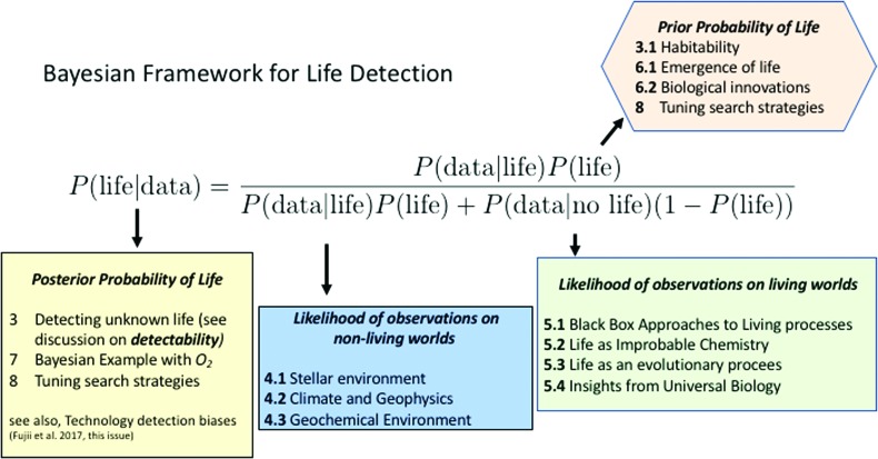
We introduce a Bayesian method for guiding future directions for detection of life on exoplanets. We describe empirical and theoretical work necessary to place constraints on the relevant likelihoods, including those emerging from better understanding stellar environment, planetary climate and geophysics, geochemical cycling, the universalities of physics and chemistry, the contingencies of evolutionary history, the properties of life as an emergent complex system, and the mechanisms driving the emergence of life. We provide examples for how the Bayesian formalism could guide future search strategies, including determining observations to prioritize or deciding between targeted searches or larger lower resolution surveys to generate ensemble statistics and address how a Bayesian methodology could constrain the prior probability of life with or without a positive detection. Key Words: Exoplanets-Biosignatures-Life detection-Bayesian analysis. Astrobiology 18, 779-824.

FIG. 1.

Conceptual diagram of the Bayesian framework for detection of exoplanet biosignatures, with section guides to this article. Color images available at www.liebertonline.com/ast

FIG. 2.

Examples of the relationship between the canonical definitions of the habitable zone and our assumptions about P(life), based on different priors. (A) A prior where a nonzero prior probability for life is limited to the canonical habitable zone. (B) A prior where a nonzero prior probability for life is not limited to the habitable zone, but where P(life)_{inside_HZ} >> P(life)_{outside_HZ}. (C) A flat prior where the prior probability for life is equally likely at any distance from the host star (not dependent on the habitable zone). By definition, the concept of a habitable zone implies that we expect P(life) > 0 (but of unknown value) for worlds within the habitable zone. See Section 6.3 for further discussion on P(life) and the habitable zone. This article focuses on detectability as opposed to habitability. Many other distributions could be considered. These examples are given to clarify how habitability might integrate into the Bayesian framework we already outline, but we do not go into further detail on this topic in this article. Color images available at www.liebertonline.com/ast

FIG. 3.

Median X-ray, FUV, and NUV excess fractional fluxes, including upper limits, as a function of stellar age for early M stars. The radiation environment changes in time and is more intense for young stars, potentially impacting the probability of life emerging P(life). Adopted from Shkolnik and Barman (2014). FUV, far-UV; NUV, near-UV. Color images available at www.liebertonline.com/ast

FIG. 4.

Modeling methodology used to explore the effects of variable volcanic–tectonic activity on planetary climate. Solid planet dynamic models of coupled mantle convection and surface tectonics (Lenardic et al., 2016) are used to map out variations in volcanic and tectonic activity over time for a range of planetary parameter values (left image). Results from the solid dynamics models are then used to generate volcanic–tectonic forcing functions for zonal energy balance climate models (Pierrehumbert, 2010) that include volcanic degassing, topography generation, and CO₂ drawdown from the atmosphere due to surface weathering (right image). Color images available at www.liebertonline.com/ast

FIG. 5.

Schematic illustrating the difference between abiotic (smooth curve) and biological (spikes) distributions of organic molecules. Nonliving systems tend to produce smooth thermodynamic distributions, whereas in living processes, only a subset of molecule species are selected (through natural selection) to form a functional set. Adopted from McKay (2011). Color images available at www.liebertonline.com/ast

FIG. 6.

Life on Earth radiated from a LUCA with a single standard genetic code. With respect to core biochemical components of life, this common ancestry leaves a sample size N = 1. However, the subsequent evolution of diverse metabolic capabilities and evolutionary lineages has resulted in diverse trajectories, allowing the possibility of mapping N = 1 to N = many, considering the varying coupled environmental and biological states over geological timescales and the number of independent convergent evolutionary innovations and transitions (only a few of which are shown for illustrative example). It is unknown how frequently these evolutionary events, including the origin of life, should be expected to occur on other worlds. Adopted from Schulze-Makuch and Bains (2017). LUCA, last universal common ancestor. Color images available at www.liebertonline.com/ast

FIG. 7.

Two different graph-theoretic representations of the same chemical network, consisting of the reactions: H + HCl → H₂ + Cl, HCl + O → Cl + OH, and HCl + OH → Cl + H₂O. Network examples adopted from Solé and Munteanu (2004). (A) Bipartite representation where both reactions and substrates are treated as nodes. (B) Unipartite representation where only substrates are treated as nodes.

FIG. 8.

A network representation of Earth's stratospheric chemical reaction network. High degree nodes are highlighted in warm tones and lower degree nodes in blue. Data are from DeMore et al. (1997). Color images available at www.liebertonline.com/ast

FIG. 9.

Empirically observed scaling laws for metabolic rate as a function of body mass exhibits three major regimes, associated with prokaryotes, protists, and metazoans (Delong et al., 2010). If these trends are universal and can be derived from an underlying common theory, it may be possible to apply the universal scaling relations to inform P(data|life) on other worlds. Adopted from Okie (2012). Color images available at www.liebertonline.com/ast

FIG. 10.

Parameters for the toy model case of detecting O₂ without additional knowledge of false positives. The prior probability is distributed between our two hypotheses: either life produced the signal (with probability p_l) or it did not (with probability 1-p_l). The likelihoods of observing O₂ are set to illustrative values of 10% for life and 20% for no life (such that nonliving worlds produce detectable atmospheric O₂ more frequently than worlds with life).

FIG. 11.

In the absence of additional contextual information, the posterior probability of life after detection of O₂ scales with our assumptions about its prior probability (which is currently unconstrained, see Section 7), see also Figure 19.

FIG. 12.

Posterior probability of life as a function of repeated independent observations of O₂ (N_observations is discrete, continuous curves are shown here to better illustrate trends). Model parameters are from Figure 10 (with ɛ = 0), using Eq. 13 for the measurement distribution as described in the text. Shown are cases for varying assumptions about the prior probability of life P(life). Color images available at www.liebertonline.com/ast

FIG. 13.

Parameters for the toy model case of detecting O₂ with additional contextual knowledge of the joint probability of O₂ and H₂O for living and nonliving worlds. The prior probability is again distributed between our two hypotheses: either life produced the signal (with total probability p_l) or it did not (with total probability 1-p_l). We assume life is much more likely in the presence of H₂O than not. The likelihoods of observing O₂ are set to illustrative values of 10% for life and 20% for no life, where nonliving processes are just as likely to yield atmospheric O₂ whether H₂O is also present or not and it is assumed life does not produce O₂ in the absence of H₂O.

FIG. 14.

Posterior probability of life as shown in Figure 12, where now additional contextual information about the co-occurrence of O₂ with H₂O is taken into account (as shown in Fig. 12, N_observations is discrete, continuous curves are shown here to better illustrate trends, and observations can be interpreted as independent measurements). Model parameters are from Figure 13, using Eq. 14. Shown are cases for varying assumptions about the prior probability of life P(life). Color images available at www.liebertonline.com/ast

FIG. 15.

Parameters for the toy model case of detecting O₂ with additional contextual information of the joint probability of O₂, H₂O, and CO for living and nonliving worlds. The prior probability is again distributed between our two hypotheses, either life produced the signal (with total probability p_l) or it did not (with probability 1-p_l): we assume life is much more likely in the presence of H₂O than not, and uniformly distributed over worlds with CO. The likelihoods of observing O₂ are set to illustrative values of 10% for life and 20% for no life, where nonliving processes are most likely to support atmospheric O₂ when H₂O and CO are also present, and living processes are most likely to support atmospheric O₂ when H₂O is present but CO is not. Highlighted in blue is the case where D > 1, i.e., P(O₂|life) > P(O₂|no life).

FIG. 16.

Posterior probability of life as shown in Figures 12 and 14, where now additional contextual information about the co-occurrence of O₂ with H₂O and CO is taken into account (as shown in Fig. 12, N_observations is discrete, continuous curves are shown here to better illustrate trends, and observations can be interpreted as independent measurements). Model parameters are from Figure 15, using Eq. 14. Shown are cases for varying assumptions about the prior probability of life P(life). Color images available at www.liebertonline.com/ast

FIG. 17.

Seasonal variation in pCO₂ as an example where we might expect P(data|life) >> P(data|abiotic), leading into an enhanced posterior probability for life. Volume mixing ratio measurements CO₂ are sourced from the NOAA at Mauna Loa, Hawaii, for the 1995–2000 time interval (Thoning et al., 2015). The seasonal change in CO₂ in the northern hemisphere is mostly reflective of the seasonal growth and decay/senescence of land-based vegetation (Keeling et al., 1996). These data were obtained from the NOAA's Earth System Research Laboratory (https://www..esrl.noaa.gov/). NOAA, National Oceanic and Atmospheric Association. Color images available at www.liebertonline.com/ast

FIG. 18.

Top: Normalized HST/WFC3 IR transmission spectra of 10 exoplanets with reported H₂O detections combined with a weighted mean to create a representative spectrum of H₂O-bearing exoplanets. Bottom: Comparison of representative spectrum (black) to single planet models (see Iyer et al., for details). Adopted from Iyer et al. (2016). If this turns out to be the case, the community may need to shift focus to thinking about also detecting life deterministically, by analyzing coherently averaged spectra of many candidate worlds. HST, Hubble Space Telescope; IR, infrared. Color images available at www.liebertonline.com/ast

FIG. 19.

The posterior probability of life after detection of O₂ will depend on the likelihood the observed signal can be produced abiotically. If life is not common (e.g., P(life) <0.1, vertical gridline), even in cases where uninhabited worlds rarely produce O₂ atmospheres (red curve, P(O₂|abiotic) = 0.001), detection of O₂ on a single exoplanet leaves the posterior probability of life is much less than certain (e.g., P(life|O2) < 0.9), meaning we cannot conclude the world is “very likely inhabited.” Color images available at www.liebertonline.com/ast

FIG. 20.

The posterior probability of life assuming a fraction f(O₂) of the N_exoplanets observed have detectable levels of atmospheric O₂. Shown are cases where the prior probability of life is 0.01 (A) and 0.001 (B). Color images available at www.liebertonline.com/ast

References

1. Abe Y., Abe-Ouchi A., Sleep N.H., and Zahnle K.J. (2011) Habitable zone limits for dry planets. Astrobiology 11:443–460 - PubMed
1. Abe Y., Numaguti A., Komatsu G., and Kobayashi Y. (2005) Four climate regimes on a land planet with wet surface: effects of obliquity change and implications for ancient Mars. Icarus 178:27–39
1. Airapetian V.S., Glocer A., Gronoff G., Hebrard E., and Danchi W. (2016) Prebiotic chemistry and atmospheric warming of early Earth by an active young Sun. Nat Geosci 9:452–455
1. Allakhverdiev S.I., Kreslavski V.D., Zharmukhamedov S.K., Voloshin R.A., Korol'kova D.V., Tomo T., and Shen J.R. (2016) Chlorophylls d and f and their role in primary photosynthetic processes of cyanobacteria. Biochemistry (Mosc) 81:201–212 - PubMed
1. Amaral-Zettler L.A., Zettler E.R., Theroux S.M., Palacios C., Aguilera A., and Amils R. (2011) Microbial community structure across the tree of life in the extreme Rio Tinto. ISME J 5:42. - PMC - PubMed
Publication types