Slice-level diffusion encoding for motion and distortion correction

Abstract

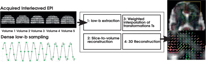
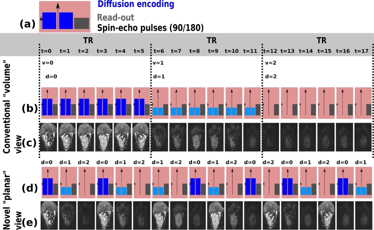
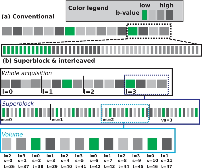
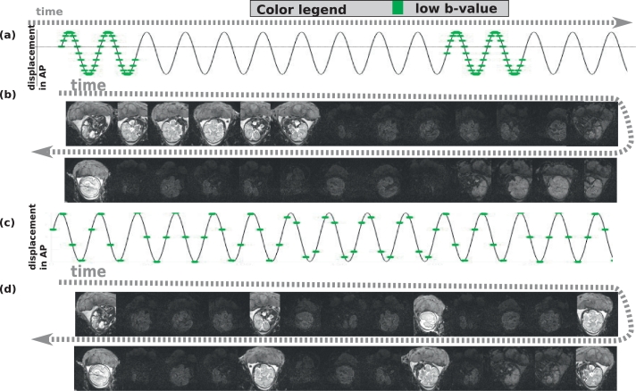
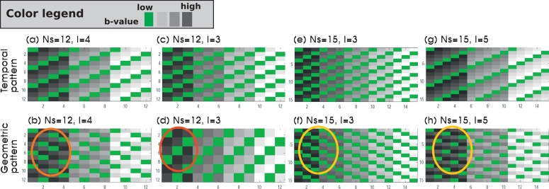
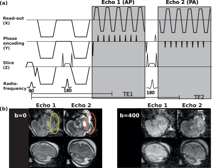
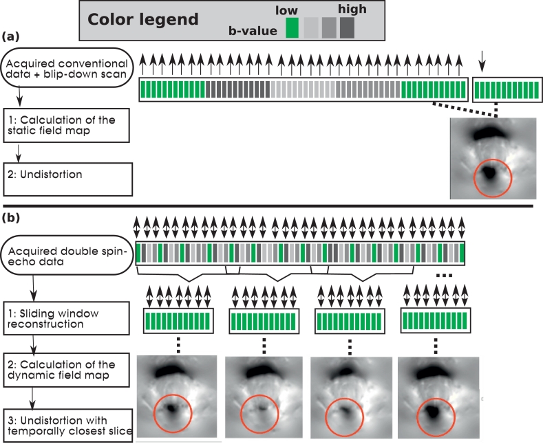
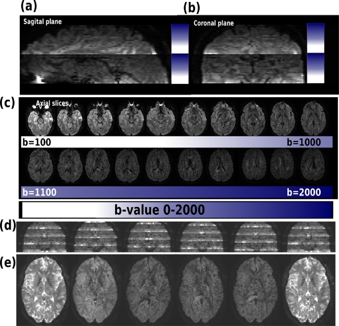
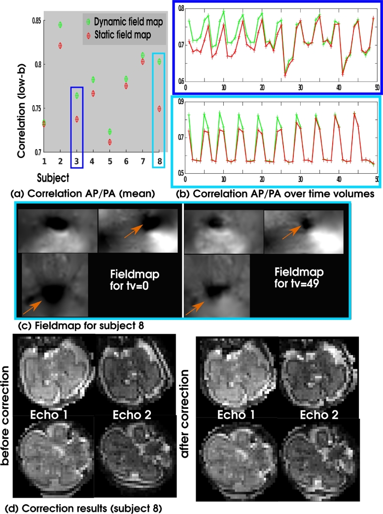
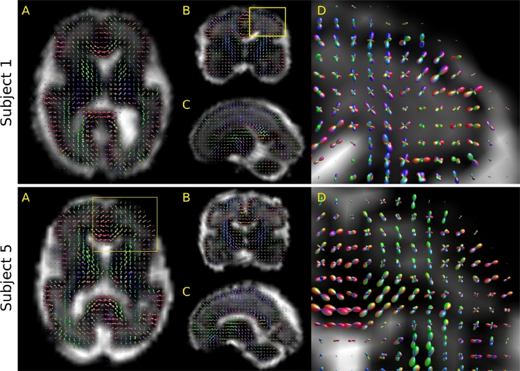
Advances in microstructural modelling are leading to growing requirements on diffusion MRI acquisitions, namely sensitivity to smaller structures and better resolution of the geometric orientations. The resulting acquisitions contain highly attenuated images that present particular challenges when there is motion and geometric distortion. This study proposes to address these challenges by breaking with the conventional one-volume-one-encoding paradigm employed in conventional diffusion imaging using single-shot Echo Planar Imaging. By enabling free choice of the diffusion encoding on the slice level, a higher temporal sampling of slices with low b-value can be achieved. These allow more robust motion correction, and in combination with a second reversed phase-encoded echo, also dynamic distortion correction. These proposed advances are validated on phantom and adult experiments and employed in a study of eight foetal subjects. Equivalence in obtained diffusion quantities with the conventional method is demonstrated as well as benefits in distortion and motion correction. The resulting capability can be combined with any acquisition parameters including multiband imaging and allows application to diffusion MRI studies in general.

Keywords: Diffusion; EPI; Foetal imaging; MRI; Microstructure; Motion correction.

Graphical abstract

Fig. 1

A schematic illustration of the acquisition scheme for one EPI slice is depicted in (a), consisting of the diffusion encoding in blue, the pulses required for the spin echo in black and the read-out train in gray. (b-c) depict a conventional volume-wise acquisition and (d-e) the proposed slice-wise acquisition. The chosen parameters are $N_s=6,$$N_d=3$. Thereby, (b) and (d) are schematics and (c) and (e) depict exemplary axial foetal brain images. (For interpretation of the references to colour in this figure legend, the reader is referred to the web version of this article.)

Algorithm 1

Calculate encoding per slice.

Fig. 2

The structure of the conventional EPI sequence (in (a)) and the proposed Superblock & Interleaving (in (b)) are depicted. In (a) the whole acquisition is shown together with a zoom into the last four volumes in the second row. In (b), a whole acquisition ($N_s=12,N_d=16,L=4$ is shown in the first row. The second row shows a zoom into the superblock $l=3$. Finally, in the third row, volume $vs=2$ within this superblock is shown together with all relevant parameters (i, s, t).

Fig. 3

The distribution of the low-b slices is illustrated schematically for conventional (a-b) and superblock and interleaved (c-d) acquisition. Thereby, the displacement in anterior-posterior direction originating from a (simplified) exemplary breathing pattern is illustrated schematically in (a) and (c) in black. In green, the temporal indices of low-b slices are indicated. In (b) and (d) slices obtained at sub-sampled temporal locations along (a) and (c) are schematically depicted to illustrate the temporal sampling density of low-b slices. (For interpretation of the references to colour in this figure legend, the reader is referred to the web version of this article.)

Fig. 4

Illustrations of the temporal (first row, a,c,e,g) and spatial (second row, b,d,f,h) patterns of low-b (green) and high-b (gray) slices are given. The same odd-even slice acquisition order [0,2,4,6.1,3,5,7.] is used for all. The varied parameters include the number of slices N_s: 12 in (a–d) and 15 in (e–h) and the superblock length L: 4 in (a–b), 3 in (c–d), 3 in (e–f) and 5 in (g–h). The coloured circles mark a suboptimal (red), non-uniform (orange) and to uniformly spread and optimal patterns (yellow). (For interpretation of the references to colour in this figure legend, the reader is referred to the web version of this article.)

Fig. 5

(a) Sequence diagram (simplified) of the double spin-echo sequence illustrating the gradient objects on Read-out (X), phase encoding (Z) and slice (Z) axis as well as radio-frequency pulses. (b) Acquired echoes with opposed phase encoding and thus equal-opposite distortions. (For interpretation of the references to colour in this figure legend, the reader is referred to the web version of this article.)

Fig. 6

The postprocessing step required to correct for geometric distortions is depicted. In (a), a conventional technique is depicted: The dMRI scan acquired with one phase encoding direction (here AP) is complemented with a subsequent single b=0 volume with opposed phase encoding direction (here PA). Correction consists of (1) the calculation go a static field map and subsequent (2) correction of all volumes using this map. In (b) the proposed approach based on double-spin echo Superblock & Interleaving data is depicted: (1)Sliding window reconstruction extracts b=0 volumes throughout the dataset. These are used to calculate (2) dynamic field maps for all time steps which are finally (3) used to correct every slice with the temporally closest map.

Fig. 7

(a) Schema of the proposed postprocessing of the Superblock & Interleaving data. The first row, consisting only of step sorting sorts the data to a conventional volume-view data set. In the second row, a four-step pipeline including motion correction is depicted. In (b)–(d), the weighting approach is illustrated. (b) Depictes the b0 result as obtained after super-resolution reconstruction, (c) the derived brain mask and (d) the obtained number of voxels within the mask as input for the calculation of the weights.

Fig. 8

Results from the simulated breathing experiment are depicted. In (a), the obtained motion free volume is shown in sagittal, coronal and transverse plane. In (b), the simulated motion patterns for different repetition times (TR=3sec first row and TR=12sec second row) and different interleave patterns (L=2 first column, L=4 second column and L=8 in the third column) are shown. All capture the time frame of two subsequent volumes, the red dots illustrate the temporal acquisition order of the low-b data. (For interpretation of the references to colour in this figure legend, the reader is referred to the web version of this article.)

Fig. 9

Results are presented from the phantom experiment. Thereby (a) illustrates the acquired data in coronal plane for the superblock scheme. (b) shows the data after sorting to conventional volumes in coronal view. In (c) the conventional data is displayed equally in coronal view. Sorted superblock and acquired conventional data at a mid-stack location in the axial plane is given in (e) and (f). Finally in (d and g) he difference between conventional and superblock is shown (scale 5% of the original data) in coronal (d) and axial (g) view.

Fig. 10

Results are presented from the healthy adult experiment. Thereby (a) illustrates the data in reformatted coronal plane for the interleaved acquisition. (b) shows the data after sorting to conventional volumes in coronal view. In (c) the conventional data is displayed equally in coronal view. Obtained ADC (d) and FA (e) maps are given for both acquisition types. Bland-Altmann plots for another subject are given in (f)–(i): Thereby the results from the conventional vs. interleaved experiments are given for ADC and FA in (f) and (g), Bland-Altman plots for the conventional vs. repeat conventional in (h) and (i) using all voxels within the brain mask.

Fig. 11

Results from the (a–c) b-value sweep experiment and the multiband acquisition (d–f) are shown on an adult brain. The sweep results are displayed reformatted in (a) sagittal and (b) coronal plane. (c) visualizes axial slices ranging from b=0 (left) to b=2000 (right). The reconstructed multiband data in coronal (d) and mid-stack axial orientation (e) is given.

Fig. 12

Resulting y-displacement curves overlaid over the sampled respiratory displacement curve are given exemplary for an acquisition with $L=4$. Thereby, the input displacement (ground truth) is given in blue, the transformation parameters obtained after registration of the low-b slices in red, and the interpolated transformation parameters for all slices in black. The green circle focuses on an outlier in the estimated transformations. It corresponds to a $b=0$ slice, located at the border of the spatial volume. The employed weighting strategy did not include these transformations in the interpolation routine. (For interpretation of the references to colour in this figure legend, the reader is referred to the web version of this article.)

Fig. 13

Results from distortion correction using the dynamic maps. (a) Mean over the correlations between AP/PA images for all low-b volumes are shown for the dynamic field map (green) vs. the static fieldmap acquired at the acquisition end (red). (b) The correlation for every diffusion weighting is shown for both corrections for subject 3 and 8. (c) Fieldmaps from the acquisition start and end and (d) correction results are shown for subject 8. (For interpretation of the references to colour in this figure legend, the reader is referred to the web version of this article.)

Fig. 14

Orientation distribution functions (ODFs) overaid onto the estimated free water fraction in subjects 1 and 5. (A-C) Axial, coronal, and sagittal slices through the brain, rendered off-axis w.r.t. the acquisition. (D) Magnified ODFs from the yellow frame. (For interpretation of the references to colour in this figure legend, the reader is referred to the web version of this article.)

References

1. Aksoy M., Forman C., Straka M., Skare S., Holdsworth S., Hornegger J., Bammer R. Real-time optical motion correction for diffusion tensor imaging. Magn. Reson. Med. 2011;66(2):366–378. - PMC - PubMed
1. Alexander D.C., Hubbard P.L., Hall M.G., Moore E.A., Ptito M., Parker G.J., Dyrby T.B. Orientationally invariant indices of axon diameter and density from diffusion MRI. Neuroimage. 2010;52(4):1374–1389. - PubMed
1. Andersson J.L.R., Skare S., Ashburner J. How to correct susceptibility distortions in spin-echo echo-planar images: application to diffusion tensor imaging. Neuroimage. 2003;20(2):870–888. - PubMed
1. Andersson J.L.R., Sotiropoulos S.N. An integrated approach to correction for off-resonance effects and subject movement in diffusion MR imaging. Neuroimage. 2015;in press - PMC - PubMed
1. Assaf Y., Blumenfeld-Katzir T., Yovel Y., Basser P.J. Axcaliber: a method for measuring axon diameter distribution from diffusion MRI. Magn. Reson. Med. 2008;59(6):1347–1354. - PMC - PubMed
Publication types