Serial dependence in the perception of visual variance

Abstract

The recent history of perceptual experience has been shown to influence subsequent perception. Classically, this dependence on perceptual history has been examined in sensory-adaptation paradigms, wherein prolonged exposure to a particular stimulus (e.g., a vertically oriented grating) produces changes in perception of subsequently presented stimuli (e.g., the tilt aftereffect). More recently, several studies have investigated the influence of shorter perceptual exposure with effects, referred to as serial dependence, being described for a variety of low- and high-level perceptual dimensions. In this study, we examined serial dependence in the processing of dispersion statistics, namely variance-a key descriptor of the environment and indicative of the precision and reliability of ensemble representations. We found two opposite serial dependences operating at different timescales, and likely originating at different processing levels: A positive, Bayesian-like bias was driven by the most recent exposures, dependent on feature-specific decision making and appearing only when high confidence was placed in that decision; and a longer lasting negative bias-akin to an adaptation aftereffect-becoming manifest as the positive bias declined. Both effects were independent of spatial presentation location and the similarity of other close traits, such as mean direction of the visual variance stimulus. These findings suggest that visual variance processing occurs in high-level areas but is also subject to a combination of multilevel mechanisms balancing perceptual stability and sensitivity, as with many different perceptual dimensions.

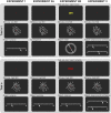
Figure 1

Experiments 1–3: Structure. In all experiments, each trial presented a random-dot kinematogram of a certain mean and variance (standard deviation, StD) in the motion trajectories of its component dots. In the example, Trials n − 1 and n have low and high StD values, respectively. Experiment 1 required variance (StD) reports for each trial, using a visual analogue scale. Experiment 2 interleaved two thirds of trials in which variance reports were required and one third in which either no response (Experiment 2A) or mean trajectory estimation (Experiment 2B) was required. In Experiment 2B the trial type was precued, so that the label “DIR” or “RAN” at the beginning of each trial indicated whether a mean or variance judgment was required for that trial. Experiment 3 required subjective confidence ratings following variance reports, using a similar visual analogue scale.

Figure 2

Experiment 1. (A) Distribution of responses by StD_n and eccentricity. The height of the bars represents the mean, and the error bars the between-subjects standard error. (B) Normalized relative error in current response (zRE_n) as a function of the StD presented in the previous trial (StD_n−1). The relative error, defined as RE_n = (R_n − StD_n)/StD_n, has been normalized by the distribution of errors provided by each subject for the current StD_n; thus, a positive zRE_n means a larger report in that trial than the participant's average for that stimulus level, and conversely a negative zRE_n indicates a lower-than-average score—that is, sign is not necessarily related to comparison with veridical StD_n, if the participant exhibits a systematic bias for that StD_n. Consequently, plotting zRE_n reports by StD_n−1 allows examination of any possible bias in relation to previous-trial StD_n−1, beyond any unrelated source of bias. The error bars represent the between-subjects standard error. The ascending slope of the plots indicates a positive bias associated with StD_n−1, for both foveal and peripheral presentations; relative overestimation occurs for larger StD_n−1. (C) Response bias associated with StD presented in recent history. Each data point represents the fixed-effects coefficient estimate (B) in a Bayesian linear mixed-effects model for the association between the StD presented in Trials n − 1 to n − 10 (StD_n−t, t = 1, …, 10) and the normalized response error in the current trial. The value of the B coefficient represents the linear slope between the past StD at a certain trial position (StD_n−t) and the normalized response error provided in the current trial—that is, the variation (in z scores) observed on the current response (regardless of the presented StD), when StD_n−t was increased by 1°. A positive B represents an attractive bias (ascending slope), and a negative B a repulsive bias (descending slope). The error bars depict the 95% credible intervals for the value of the B coefficient.

Figure 3

Experiment 2. (A, B) Normalized relative error in current response (zRE_n) as a function of the StD presented in the previous trial (StD_n−1), plotted separately by Trial n − 1 type: (A) response versus no-response (Experiment 2A); (B) RAN versus DIR (Experiment 2B). The error bars represent the between-subjects standard error. Both response and no-response trials are associated with a positive bias by Trial n − 1, as suggested by the ascending plot lines in (A), whereas in (B), only RAN trials elicit such positive serial dependence. (C, D) Fixed-effects coefficient estimates in 20 Bayesian linear mixed-effects models with StD_n−t (t = 1, …, 10) as predictor of current response (zRE_n), modeled separately by Trial n − t type: (C) response versus no-response (Experiment 2A); (D) RAN versus DIR (Experiment 2B). Since the dependent variable is the current variance (randomness) judgment, Trial n is always a response (C) or RAN (D) trial. The error bars represent the 95% credible intervals for the true value of the coefficient.

Figure 4

Experiment 3. (A) Confidence scores (C_n) by StD_n plotted separately by eccentricity. (B, C) Normalized relative error in current response (zRE_n) as a function of the StD presented in the previous trial (StD_n−1), plotted separately by confidence reported in (B) the current or (C) the previous trial. Confidence scores have been binned into tertiles according to each participant's distribution of reports. The error bars represent the between-subjects standard error. The plots in (B) are all ascending and roughly parallel, indicating that current confidence does not modulate serial dependence by previous-trial StD. Conversely, when considering confidence reported in the previous (n − 1) trial (C), we observe drastically different slopes: While the high-confidence plot (upper tertile) has a clear ascending slope indicative of a positive bias, the middle-tertile plot is only mildly positive, and the lower-tertile plot is slightly descending, suggesting a negative bias away from low-confidence n − 1 trials. (D) Fixed-effects coefficient estimates in 30 Bayesian linear mixed-effects models with StD_n−t (t = 1, …, 10) as predictor of current response (zRE_n), modeled separately by confidence reported in Trial n − t (C_n−t), binned into tertiles. The error bars represent the 95% credible intervals for the true value of the coefficient. As suggested for Trial n − 1 in (C), the size and direction of the bias associated with each trial position depends on the confidence reported in that position, so that the bias will be more negative (or less positive) the lower the reported confidence, within the general trend of an increasingly negative (less positive) bias as we move backward in history.

Figure 5

Comparison between Experiments 1 and 3. Both experiments have the same design except for the requirement of a confidence report (in addition to a variance report) per trial in Experiment 3. This also makes the interstimulus time longer, on average, for Experiment 3 compared to Experiment 1. (A) Fixed-effects coefficient estimates in 20 Bayesian linear mixed-effects models with StD_n−t (t = 1, …, 10) as predictor of current response (zRE_n), with the data of Experiments 1 and 3 modeled separately. The error bars represent the 95% credible intervals for the true value of the coefficient. The shift toward negative coefficient estimates takes place at earlier trial positions in Experiment 3. (B) Fixed-effects coefficient estimates for the StD_n−t × time_n,n−t and StD_n−t × C-report_n−t interactions in 10 Bayesian linear mixed-effects models for prediction of zRE_n, with StD_n−t, time_n,n−t, C-report_n−t, and all interactions as putative predictors. The variable time_n,n−t reflects the time between onsets of the stimuli in Trials n − t (t = 1, …, 10) and n. C-report_n−t is a binary factor indicating whether confidence reports were made in all trials between n − t and n or in none, regardless of the content of the reports (i.e., the amount of confidence). A negative interaction term with StD_n−t indicates a less positive (more negative) serial-dependence effect in relation with longer time or the requirement of an additional confidence report per trial. While credible intervals contain zero in most instances, there is a predominance of negative estimates up to n − 5, which could suggest a causal role for both time and the additional confidence report in terms of promoting an earlier reversal of the bias in Experiment 3 compared to Experiment 1.

References

1. Alais, D., Ho, T., Han, S.. (2017). A matched comparison across three different sensory pairs of cross-modal temporal recalibration from sustained and transient adaptation. i-Perception, 8 4, 1– 18, https://doi.org/10.1177/2041669517718697. - DOI - PMC - PubMed
1. Albrecht, A. R., Scholl, B. J.. (2010). Perceptually averaging in a continuous visual world: Extracting statistical summary representations over time. Psychological Science, 21 4, 560– 567, https://doi.org/10.1177/0956797610363543. - DOI - PubMed
1. Alvarez, G. A. (2011). Representing multiple objects as an ensemble enhances visual cognition. Trends in Cognitive Sciences, 15 3, 122– 131, https://doi.org/10.1016/j.tics.2011.01.003. - DOI - PubMed
1. Alvarez, G. A., Oliva, A.. (2009). Spatial ensemble statistics are efficient codes that can be represented with reduced attention. Proceedings of the National Academy of Sciences, USA, 106 18, 7345– 7350, https://doi.org/10.1073/pnas.0808981106. - DOI - PMC - PubMed
1. Ariely, D. (2001). Seeing sets: Representation by statistical properties. Psychological Science, 12 2, 157– 162. - PubMed
Publication types
LinkOut - more resources