Exploiting limited valence patchy particles to understand autocatalytic kinetics

Abstract

Autocatalysis, i.e., the speeding up of a reaction through the very same molecule which is produced, is common in chemistry, biophysics, and material science. Rate-equation-based approaches are often used to model the time dependence of products, but the key physical mechanisms behind the reaction cannot be properly recognized. Here, we develop a patchy particle model inspired by a bicomponent reactive mixture and endowed with adjustable autocatalytic ability. Such a coarse-grained model captures all general features of an autocatalytic aggregation process that takes place under controlled and realistic conditions, including crowded environments. Simulation reveals that a full understanding of the kinetics involves an unexpected effect that eludes the chemistry of the reaction, and which is crucially related to the presence of an activation barrier. The resulting analytical description can be exported to real systems, as confirmed by experimental data on epoxy-amine polymerizations, solving a long-standing issue in their mechanistic description.

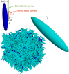
Fig. 1

The model. Graphic description of the two types of hard ellipsoids composing the simulated system, and snapshot of the system in the initially monomeric state. The centers of the small (yellow) spheres locate the bonding sites on the surface of the hard-core particle. The site–site interaction, sketched as a function of the inter-site distance r, is modeled as an attractive square-well potential complemented by a repulsive entry barrier of finite height (in red) and an infinite repulsive exit barrier (in green). Bonds can be formed only between small (blue) and big (cyan) particles

Fig. 2

Kinetics of autocatalytic reactions. Kinetic curves, p versus time, at fixed temperature and energy barrier (βΔU₀ = 4) for different values of autocatalytic strength ξ, as indicated. Time is scaled by ${\mathrm{e}}^{\beta \mathrm{\Delta }{U}_{\mathrm{0}}}$ to highlight speed-up of the reaction due to autocatalysis. The profile of the site–site potential for bond formation, including its qualitative behavior during reaction, is sketched in the inset as a function of the inter-site distance r (Methods section)

Fig. 3

Barrier effect. Reaction rate dp/dt scaled by (1 − p)²e^−βΔU, for different values of energy barrier, as indicated. For each βΔU, symbols are mean ± SEM of the results of 40 independent simulation runs. The solid line is the description of the data in the case without barrier, using dp/dt = k_overall(1 − p)², with k_overall = (1/k_c + 1/k_dD)⁻¹, where D is the p-dependent average diffusion coefficient of a particle in the system (see next Fig. 4a)

Fig. 4

System’s diffusivity and cluster size distribution. a Average diffusion coefficient D determined from the particle mean-squared displacements (Methods section) for the system without barrier and with barrier. The p dependence is described by D = D₀[(p₀ − p)/p₀]^γ with γ = 2.69, p₀ = 0.902, and D₀ the diffusion in the initially unbonded state. b Distribution n(s) of the size s of clusters present at p = 0.2 in systems with fixed barrier (as indicated), providing evidence that the cluster size distribution is independent of both presence and height of the barrier. c Cluster size distribution during non-autocatalytic reaction with barrier βΔU = 4 (closed symbols) and during autocatalytic reaction of equal initial barrier (open symbols). Solid lines represent Flory-Stockmayer predictions. The comparison is shown at three values of p, before and after percolation (p_gel = 0.5). No difference emerges, providing evidence that the distribution of clusters at any given p is independent from the autocatalytic nature of the reaction. d Populations of clusters of different size, from monomers to tetramers, in the system reacted up to p_gel = 0.5. In each population, big and small particles are distinguished by color

Fig. 5

Dependence of non-autocatalytic kinetics on the height of barrier. a Comparison between the kinetics of the model with barrier and without barrier. The data are fitted by dp/dt = k_overall(1 − p)², where k_overall = (1/k_chem + 1/k_diff)⁻¹ with k_chem and k_diff given by Eq. 2, by weighting each datapoint with its standard error (not shown since within the symbol size). By using k_c = 4.56⋅10⁻³ and k_d = 1.015 obtained with βΔU = 0, and D(p) obtained from the mean-squared displacement, the fit only adjusts two parameters, n and k₀, for each βΔU > 0. The uncertainty of the best-fit parameters is reported in b and c with error bars. b The barrier dependence of the exponent n is analytically described by n = (n₀ − n_∞)e^−βΔU + n_∞, with n₀ = 2.01 ± 0.01 and n_∞ = 1.830 ± 0.006. c The barrier dependence of k₀, over the investigated range, is approximated by k₀ = e^bβΔU, with b = 0.31 ± 0.02

Fig. 6

Description of the autocatalytic kinetics. The p dependence of the rate dp/dt (scaled by ${\mathrm{e}}^{-\beta \mathrm{\Delta }{U}_{\mathrm{0}}}$ to facilitate comparison) at different autocatalytic strengths ξ and initial energy barriers βΔU₀. The solid lines are the predicted kinetics, i.e., dp/dt = k_overall(1 − p)² where k_overall = (1/k_chem + 1/k_diff)⁻¹, with k_chem and k_diff given by Eqs. 2 and 4, and using D(p) obtained from the mean-squared displacement. All the parameters are known from non-autocatalytic reactions. The dotted lines (in some cases they cannot be distinguished from the solid lines) represent the best-fit of the simulation data with k_chem replaced by the Kamal’s rate constant, i.e., k_chem = (k₁ + k₂p^M)(1 − p)^N−2 with k₁, k₂, M, and N free-parameters independent of p. The values of M, N, and k₂/k₁ associated to each dotted line is indicated. Below each frame, in the same color as the symbols, the residues with respect to the predicted kinetics are shown as solid lines, and with respect to the best-fitted Kamal equation as dotted lines. Different panels refer to different values of βΔU₀

Fig. 7

Qualitative comparison with experimental data. Symbols: reaction rate scaled by ${\mathrm{e}}^{-\beta {\Delta U}_0}$ obtained from simulation Colored lines: experimental data for stoichiometric formulations of epoxy–amine resins, scaled by an arbitrary factor. Discrepancy in the high p region depends on the different p dependence of the diffusion coefficient in experimental reality with respect to the simulation model

Fig. 8

Quantitative comparison with experimental data. Colored symbols are experimental data—taken from a ref. , b ref. , c–f ref. — for the kinetics of diglycidyl ether of bisphenol-A (DGEBA) reacted at different temperatures with different amines (1,3-phenylenediamine (mPDA), 4-4′(1,3-phenylene-diisopropylidene) bisaniline (BSA), 4,4′-diamino-3,3′-dimethyldicyclohexylmethane (3DCM), diethylenetriamine (DETA), cyclohexylamine (CHA), 4,4′-diaminodiphenylmethane (DDM)). Each curve corresponds to a different T of reaction. The red lines are obtained by fitting the data at all temperatures simultaneously using dp/dt = (1/k_chem + 1/k_diff)⁻¹(1 − p)², where $k_{\mathrm{chem}}=\left(A{\mathrm{e}}^{-\beta \mathrm{\Delta }{U}_{\mathrm{c}}}+B{\mathrm{e}}^{-\beta \mathrm{\Delta }{U}_{\mathrm{a}}}p\right){\left(1-p\right)}^{n-2}$ with $n=n_{\infty }+\left(n_0-n_{\infty }\right)\left({\mathrm{e}}^{-\beta \mathrm{\Delta }{U}_{\mathrm{c}}}+\left(B∕A\right){\mathrm{e}}^{-\beta \mathrm{\Delta }{U}_{\mathrm{a}}}p\right)$, and k_diff = k_dτ^−λ with τ the p-dependent structural relaxation time, experimentally measured at each T. Assuming n₀ = 2, the simultaneous fit procedure over different isotherms adjusts for each system seven parameters, i.e., ΔU_c, ΔU_a, n_∞, A, B, k_d, and λ. The black lines are obtained by fitting the same data at each T separately, with k_chem replaced by the Kamal’s rate constant, and k_diff = k_dτ^−λ as in our strategy, and thus using $4\mathbb{N}+2$ parameters, with $\mathbb{N}$ the number of isotherms. The behavior of $k_1=A{\mathrm{e}}^{-\beta \mathrm{\Delta }{U}_{\mathrm{c}}}$ and $k_2=B{\mathrm{e}}^{-\beta \mathrm{\Delta }{U}_{\mathrm{a}}}$ corresponding to the two fit strategies is reported in the Arrhenius plot, respectively, with blue lines and black symbols

References

1. Bissette AJ, Fletcher SP. Mechanisms of autocatalysis. Angew. Chem. Int. Ed. 2013;52:12800–12826. doi: 10.1002/anie.201303822. - DOI - PubMed
1. Ruiz-Mirazo K, Briones C, de la Escosura A. Prebiotic systems chemistry: new perspectives for the origins of life. Chem. Rev. 2014;114:285–366. doi: 10.1021/cr2004844. - DOI - PubMed
1. Nghe P, et al. Prebiotic network evolution: six key parameters. Mol. Biosyst. 2015;11:3206–3217. doi: 10.1039/C5MB00593K. - DOI - PubMed
1. Semenov SN, et al. Autocatalytic, bistable, oscillatory networks of biologically relevant organic reactions. Nature. 2016;537:656–660. doi: 10.1038/nature19776. - DOI - PubMed
1. Dadon Z, Wagner N, Ashkenasy G. The road to non-enzymatic molecular networks. Angew. Chem. Int. Ed. 2008;47:6128–6136. doi: 10.1002/anie.200702552. - DOI - PubMed
Publication types
LinkOut - more resources