Review
. 2018 Aug 13;376(2126):20180046.
doi: 10.1098/rsta.2018.0046.

A review of Morlet wavelet analysis of radial profiles of Saturn's rings

Affiliations
Review

A review of Morlet wavelet analysis of radial profiles of Saturn's rings

Matthew S Tiscareno et al. Philos Trans A Math Phys Eng Sci. .

Abstract

Spiral waves propagating in Saturn's rings have wavelengths that vary with radial position within the disc. The best-quality observations of these waves have the form of radial profiles centred on a particular azimuth. In that context, the wavelength of a given spiral wave is seen to change substantially with position along the one-dimensional profile. In this paper, we review the use of Morlet wavelet analysis to understand these waves. When signal to noise is high and the cause of the wave is well understood, wavelet analysis has been used to solve for wave parameters that are diagnostic of local disc properties. Waves that are not readily perceptible in the spatial domain signal can be clearly identified. Furthermore, filtering in wavelet space, followed by the reverse wavelet transform, has been used to isolate the part of the signal that is of interest. When the cause of the wave is not known, comparing the phases of the complex-valued wavelet transforms from many profiles has been used to determine wave parameters that cannot be determined from any single profile. When signal to noise is low, co-adding wavelet transforms while manipulating the phase has been used to boost a wave's signal above detection limits.This article is part of the theme issue 'Redundancy rules: the continuous wavelet transform comes of age'.

Keywords: Saturn system; planetary rings; wavelet transform.


Conflict of interest statement

We declare we have no competing interests.

Figures

Figure 1.
Figure 1.
The Morlet wavelet with ω0 = 6. The solid line shows the real part, the dashed line the imaginary part. For ease of viewing, the Gaussian envelope within which the wavelet oscillates is shown as a dotted line. The wavelet translates and dilates in order to interrogate the signal at all scales (s) and locations (r). Figure from Tiscareno et al. [11].
Figure 2.
Figure 2.
(a) Synthetic density wave radial profile generated by equation (2.1) with the values of table 1, (b) wavelet phase and (c) wavelet energy. As with all wavelet plots in this paper, contours are logarithmic, with three contours to an order of magnitude, and the lowest contour level is at the square of the median error estimate for the scan (here we artificially set σ input = 0.1). The region filled with cross-hatching is the cone of influence. The dashed line is the foreknown wavenumber kDW(r) (equation (2.6)), while the solid line shows the calculated location of a wavelet ridge (equation (3.13)); here, the two diverge visibly only for r − rL  <  40 km, corresponding to ξ  <  6. Figure from Tiscareno et al. [11].
Figure 3.
Figure 3.
(a) Calculated wavelet ridge (§3g), as in figure 2c (solid line); the expected wavenumber kDW(r) (dotted line). The region of the wavelet ridge plotted in bold was used in a linear fit (dashed line); the y = 0 point is plotted as a solid diamond. (b) All three curves from figure 3a, shown as residuals with the expected wavenumber kDW(r). (c) Calculated wavelet phase formula image
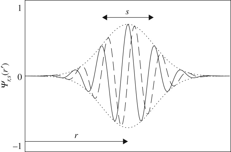
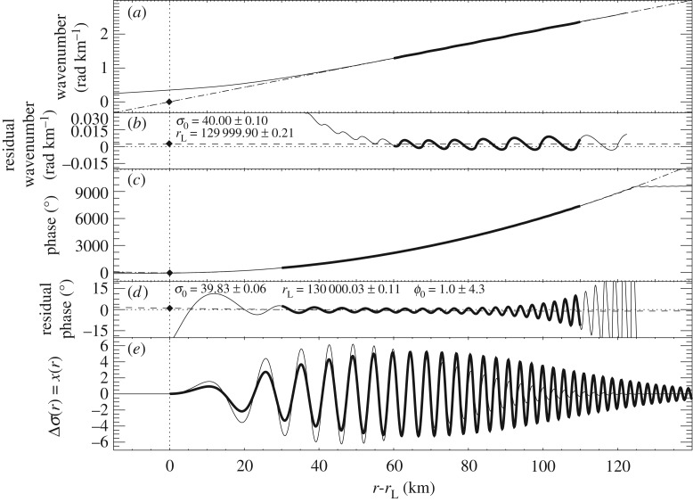
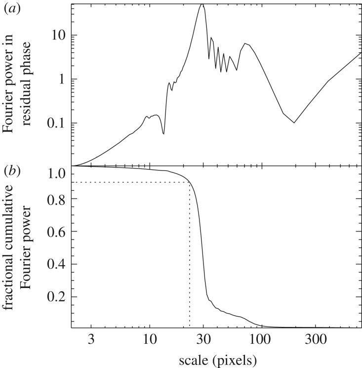
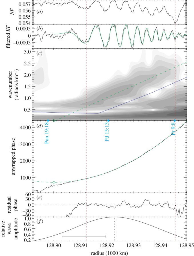
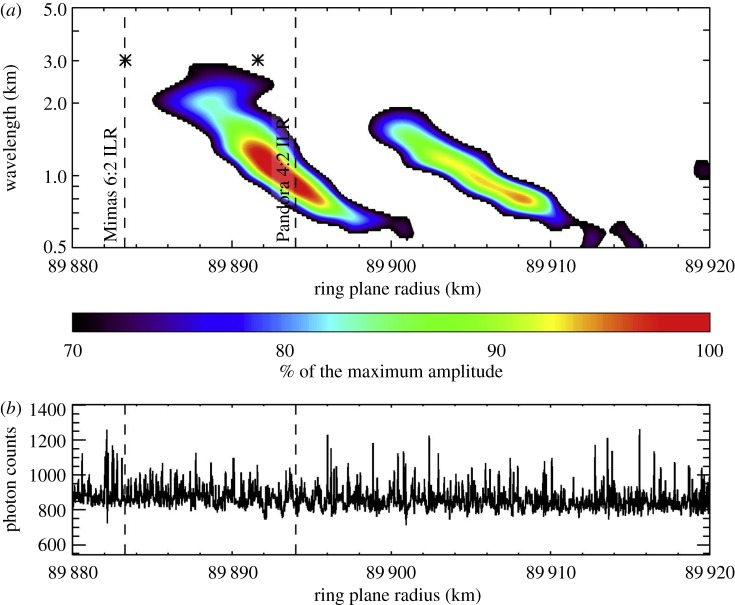
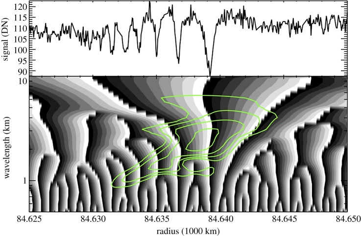
, as in figure 2b, ‘unwrapped’ to show how phase accumulates quadratically (solid line); the expected phase ϕDW(r) (dotted line). The region of formula image shown in bold was used in a quadratic fit (dashed line); the zero-derivative point is plotted as a solid diamond. (d) All three curves from figure 3c, shown as residuals with the expected phase ϕDW(r). (e) The input synthetic density wave from figure 2a (solid line); the fitted density wave, after the analysis of §4a(i), but still with randomly chosen values of ξD and AL (bold solid line). Fitted values given in the figure can be compared with the input parameters (table 1) used to generate the wave. Figure from Tiscareno et al. [11].
Figure 4.
Figure 4.
(a) The absolute value of Δσ(r) (solid line); the same curve, smoothed three times with a 22 km boxcar filter, giving the low-frequency shape of the wave envelope (bold solid line); maximum point of the latter (vertical bold dashed line). (b) The input synthetic density wave from figure 2a (solid line); the fitted density wave, after the analysis of §4a(ii), but still with randomly chosen value of AL (bold solid line). (c) The input synthetic density wave from figure 2a (solid line); the final fitted density wave, after the analysis of §4a(iii). Fitted values given in the figure can be compared with the input parameters (table 1) used to generate the wave. Figure from Tiscareno et al. [11].
Figure 5.
Figure 5.
(a) The Fourier transform of the residual phase from figure 3d. (b) The fraction of Fourier power at scales λ > λ′, for all λ′. The dotted lines show that, for our synthetic wave, 90% of the Fourier power resides at scales greater than λ90 = 22.7 pixels. Figure from Tiscareno et al. [11].
Figure 6.
Figure 6.
The density wave fitting process, illustrated using the Pan 19:18 ILR density wave, observed in Cassini image N1467345975. The two red vertical dotted lines indicate the interval used for the quadratic fit. From top to bottom: (a) radial scan, (b) high-pass-filtered radial scan, with the final fitted wave shown in green, and (c) wavelet transform of radial scan, with the blue line indicating the filter boundary, and the green dashed line indicating the fitted wave's wavenumber. (d) Unwrapped wavelet phase, with the green dashed line indicating the quadratic fit and the green open diamond indicating the zero-derivative point. (e) Residual wavelet phase, showing that the interval used for the fit is the interval in which the phase behaves quadratically. (f) Wave amplitude, the local maximum of which (vertical dotted line) gives ξD; scale bar indicates the smoothing length of the boxcar filter. Figure from Tiscareno et al. [11].
Figure 7.
Figure 7.
Location within Saturn's main ring system of figures in this paper.
Figure 8.
Figure 8.
A portion of N1560310219, from the ‘high-resolution radial scan’ 046/RDHRESSCN, shown here as an example (analysis is shown in figure 9). The nominal radial scale for this image is 0.7 km px−1. As indicated by the annotations, the ring radius (i.e. the distance from Saturn's centre) increases from bottom to top. The most prominent features in this image are the outward-propagating Prometheus 12:11 SDW and the inward-propagating Mimas 5:3 SBW. The rest of the image is pervaded by a more subtle structure that resembles the grooves on a vinyl record. Figure from Tiscareno & Harris [18].
Figure 9.
Figure 9.
Radial profile and wavelet plot for image N1560310219, continuing the example begun in figure 8. The radial profile extends across the top, and the greyscale shading in the main part of the plot indicates power in the wavelet transform (§4b). The signature of the Prometheus 12:11 SDW hangs downward from the associated cyan dashed line with a concave-up geometry [18], while the signature of the Mimas 5:3 SBW hews more closely to the associated magenta dashed line, because SBWs do not display significant nonlinearity. The ‘record grooves’ mentioned in figure 8 are here revealed to be weaker SDWs, mostly resonance with Pan (red) but some resonances with Atlas (green) and second-order resonances with Prometheus (cyan) and Pandora (dark blue). Wave models shown in bold are judged to appear in the data, while those shown as thin lines (e.g. Pan 49:48, the Janus/Epimetheus 16:13 bending waves) are not perceptible because they are overwritten by other, strong structures. All wave models in this figure use an unperturbed surface mass density σ0 = 32 g cm−2. Figure from Tiscareno & Harris [18].
Figure 10.
Figure 10.
Wavelet transform plot (top) and derived unperturbed surface mass density profile (bottom) from the Iapetus −1:0 SBW. Figures from Tiscareno et al. [17].
Figure 11.
Figure 11.
Surface mass density profile including the B ring. The filled circles are derived from the wave model fits to wavelet signatures in [18]. The filled circles in the Cassini Division (CD) correspond to individual SDWs and SBWs, while the filled circles in the A ring correspond to regions fit collectively. The solid line corresponds to the Iapetus −1:0 SBW [17]. The open squares are data points from [24], and the arrow indicates a surface mass density measurement of approximately 130 g cm−2 from the same work. The open circle is a data point from Lissauer [43], as cited in [24]. Figure from Tiscareno & Harris [18].
Figure 12.
Figure 12.
A portion of Cassini image N1467346329, showing a ‘corduroy’ pattern caused by moonlet wakes excited by Pan. Also seen are the Pandora 11:10 and Prometheus 15:14 density waves. See figure 13 for analysis. Figure from Tiscareno et al. [11].
Figure 13.
Figure 13.
Radial scan and two wavelet transforms from Cassini image N1467346329 (figure 12), showing wakes excited by Pan along with several density waves. (a) The wavelet plot, like all others in this paper, uses a central frequency ω0 = 6; (b) uses ω0 = 12, resulting in increased resolution in the spectral (y)-dimension at the expense of smearing in the radial (x)-dimension (see §3c). Density waves are clearer in (a), including the strong Pandora 11:10 and Prometheus 15:14 waves, but also the weak third-order Janus 17:14. Dashed lines indicate model density wave traces, assuming a background surface density σ0 = 40 g cm−2. Moonlet wakes excited by Pan are clearer in (b). The three dotted lines denote the frequency profiles [7] of wakes that have travelled 342°, 702° or 1062° in synodic longitude since their last encounters with Pan. Figure from Tiscareno et al. [11]. (Online version in colour.)
Figure 14.
Figure 14.
(a) Wavelet power profile of the Mimas 6:2 and Pandora 4:2 SDWs in the C ring, derived by co-adding wavelet profiles from UVIS occultations via the WWZ process. The y-axis is wavelength, rather than wavenumber as in other figures in this work. (b) One of the individual UVIS occultations from which the wavelet profile in a was computed, namely β Centauri from Rev 85. The waves are not visible by eye in this profile. Figure from Baillié et al. [22].
Figure 15.
Figure 15.
Profiles of six waves in the C ring obtained during the occultation of the star RS Cancri on Rev 80. The black profiles were obtained during ingress, while the green profiles were obtained during egress. The normal optical depth values assume the star's elevation angle above the rings is 29.96°. Note that the phase differences between the waves seen in ingress and egress are the same for the three waves found around 82 000 km. This suggests that all these waves have the same m-numbers. Figure from Hedman & Nicholson[4].
Figure 16.
Figure 16.
Profiles of six waves in the C ring obtained during the occultation of the star RS Cancri on Rev 85. The black profiles were obtained during ingress, while the green profiles were obtained during egress. Note that the phase differences between the waves seen in ingress and egress are again the same for the three waves found around 82 000 km. This implies that all these waves have the same m-numbers. The two waves found outside 84 000 km also show similar phase differences, indicating that they may have the same m-number as each other. Figure from Hedman & Nicholson [4].
Figure 17.
Figure 17.
Plot showing the wavelet amplitude and phase derived from the W84.64 wave observed by the Rev 106 RCas occultation. The top panel shows the occultation profile (in raw Data Numbers, which is proportional to transmission) as a function of radius. The bottom panel shows the wavelet phase and power as functions of radius and spatial wavelength. The wavelet phase is indicated by greyscale levels (black = − 180°, white = + 180°) while the overlaid green contours are levels of constant wavelet power. The peak wavelet power follows a diagonal ridge that corresponds to the wave's increasing wavelength with radius. Note that where the wavelet power is strong, the contours of wavelet phase are nearly vertical and correspond to the expected phase of the wave (e.g. the phase wraps from −180° to 180° at locations corresponding to sharp minima in the profile). Figure from Hedman & Nicholson [4].
Figure 18.
Figure 18.
Results of the wavelet calculations of the phase difference in wave W82.21 between the ingress and egress cuts from the Rev 85 RS Cancri occultation. The top panel shows two occultation profiles, while the middle panel shows the integrated wave power Eeff(r) between wavenumbers of 2π/(5 km) and 2π/(0.1 km). The bottom panel shows the phase difference δϕ(r) = ϕegress(r) − ϕingress(r) between these two cuts (see text for explanations of the dashed and dotted lines). Note that the average phase difference is computed using only the data where the average Eeff of the two profiles is above 0.9. The average phase difference is near 240°, which is consistent with the offset between the ingress and egress wave profiles noted in figure 16. Figure from Hedman & Nicholson [4].
Figure 19.
Figure 19.
Results of the wavelet calculations of the phase difference in wave W84.64 between the ingress and egress cuts from the Rev 85 RS Cancri occultation, following the same layout as in figure 18. In this case, the average phase difference is near 180°, which is again consistent with the ingress and egress wave profiles. Figure from Hedman & Nicholson [4].
Figure 20.
Figure 20.
Plot showing the difference between the observed and predicted values of δϕ between the ingress and egress cuts of the RS Cancri occultations for the wave W82.21 as a function of the assumed m-number, given the stipulated δλ and δt values. Different symbols correspond to different pairs of occultation cuts. Note that the residuals for both observations are close to zero when m = − 2,  − 3 and +6, so these values of m are the ones most consistent with the observed phase differences. Figure from Hedman & Nicholson [4].
Figure 21.
Figure 21.
Plot showing the difference between the observed and predicted values of δϕ between the ingress and egress cuts of the RS Cancri occultations for the wave W84.64 as a function of the assumed m-number. Note that the residuals for all three observations are close to zero when m = − 2,  + 5 and +6, so these values of m are the ones most consistent with the observed phase differences. Figure from Hedman & Nicholson [4].
Figure 22.
Figure 22.
A test of our pattern-speed determination algorithms using the Prometheus 8:7 wave in the inner A ring. (a) The RMS phase difference residuals as a function of pattern speed assuming the pattern has an m = 8, as expected for this wave. The dashed line marks the predicted pattern speed for this pattern, while the dotted line marks the pattern speed that gives the minimum variance (in this case, these two lines are almost on top of each other). (b) The residuals in the phase differences from this best-fit solution as a function of time difference between the pairs of observations. The scatter in these data likely represents residual geometrical uncertainties in the various profiles. Figure from Hedman & Nicholson [4].
Figure 23.
Figure 23.
Plots showing the RMS phase difference residuals as a function of pattern speed for each of the six waves, assuming the pattern has the indicated m-numbers. The dashed line marks the predicted pattern speed for this pattern at the resonant location provided by [22], while the dotted line is the pattern speed that gives the minimum variance in the residuals. Figure from Hedman & Nicholson [4].
Figure 24.
Figure 24.
Sample analysis of the Prometheus 7:6 wave in the A ring. The top panel shows the transmission through the A ring as a function of radius from the Rev 89 occultation by γ Crucis. The two density waves clearly visible in this profile are due to the Pandora 6:5 and Prometheus 7:6 resonances. The second panel shows the average wavelet power formula image 
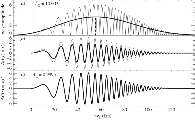
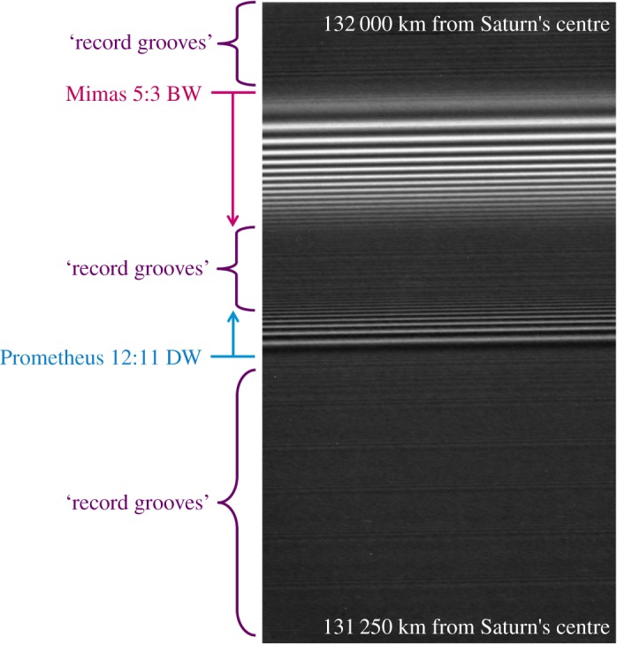
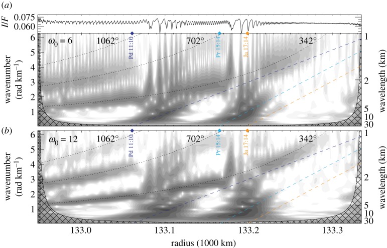
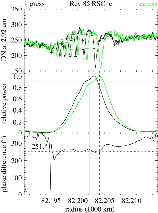
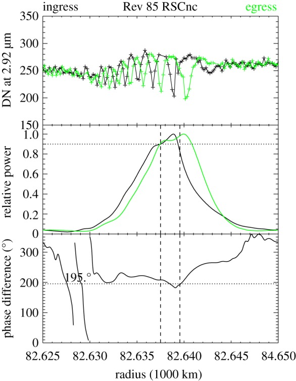
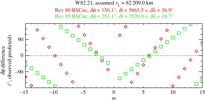
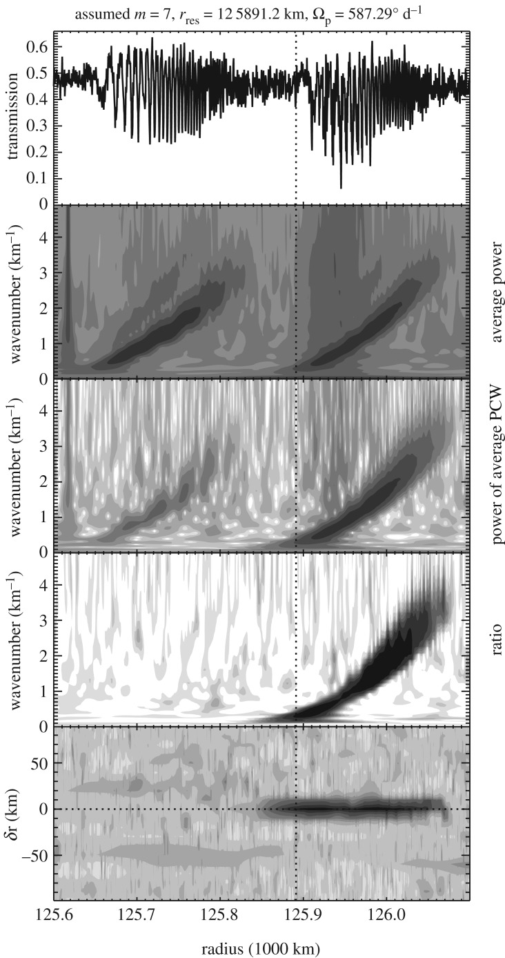
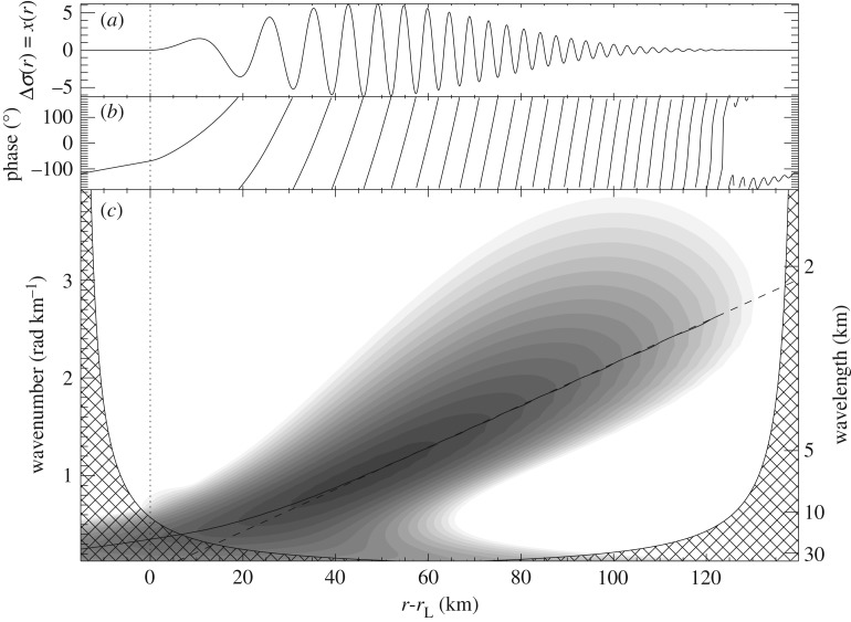
for the γ Crucis occultations, with clear diagonal bands associated with both waves. The third panel shows the power of the average phase-corrected wavelet Eϕ, assuming m = 7 and a pattern speed appropriate for the Prometheus 7:6 resonance (the exact resonance location is marked by the vertical dotted line). Note that this highlights the right-hand wave. The fourth panel shows the ratio of the above powers formula image, and shows only the signal from that wave. Finally, the bottom panel shows the peak value of formula image as a function of radius and assumed pattern speed, parametrized as a displacement δr from the expected Prometheus 7:6 resonance location (marked with a horizontal dotted line). Note that the maps of formula image and Eϕ use a common logarithmic stretch, while the maps of formula image use a linear stretch. Figure from Hedman & Nicholson [24].
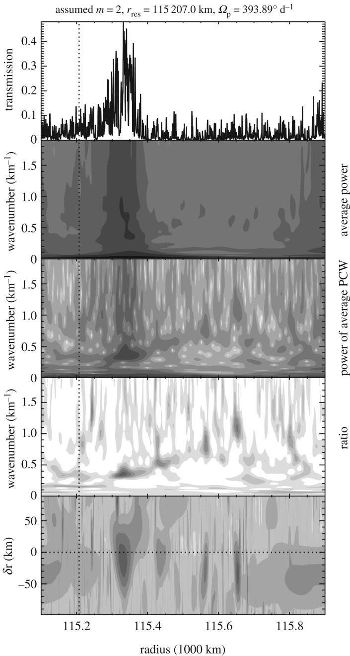
Figure 25.
Figure 25.
Wavelet analysis on the Enceladus 3:1 wave in the same format as figure 24. Unlike the test case shown in figure 24, the wave shown here was expected but has never been clearly perceived or measured before. A weak wave-like signature can be observed as a diagonal band in the ratio plot (fourth panel) that extends between 115 300 and 115 650 km in radius and between 0.5 and 1.0 km−1 in wavenumber. The bottom panel demonstrates that this signal only occurs when the assumed pattern speed is fairly close to the expected pattern speed of the density wave (i.e. where δr is close to zero). Figure from Hedman & Nicholson [24].

References

    1. Lin CC, Shu FH. 1964. On the spiral structure of disk galaxies. Astrophys. J. 140, 646–655. (10.1086/147955) - DOI
    1. Goldreich P, Tremaine S. 1982. The dynamics of planetary rings. Ann. Rev. Astron. Astrophys. 20, 249–283. (10.1146/annurev.aa.20.090182.001341) - DOI
    1. Shu FH. 1984. Waves in planetary rings. In Planetary rings (eds R Greenberg, A Brahic), pp. 513–561. Tucson, AZ: University of Arizona Press.
    1. Hedman MM, Nicholson PD. 2013. Kronoseismology: Using density waves in Saturn's C ring to probe the planet's interior. Astron. J. 146, 12 (10.1088/0004-6256/146/1/12) - DOI
    1. Hedman MM, Nicholson PD. 2014. More Kronoseismology with Saturn's rings. Mon. Not. R. Astron. Soc. 444, 1369–1388. (10.1093/mnras/stu1503) - DOI

LinkOut - more resources