. 2019 Mar;66(3):609-622.
doi: 10.1109/TBME.2018.2852306. Epub 2018 Jul 2.

Prediction of Abdominal Aortic Aneurysm Growth Using Dynamical Gaussian Process Implicit Surface

Prediction of Abdominal Aortic Aneurysm Growth Using Dynamical Gaussian Process Implicit Surface

Huan N Do et al. IEEE Trans Biomed Eng. 2019 Mar.

Abstract

Objective: We propose a novel approach to predict the Abdominal Aortic Aneurysm (AAA) growth in future time, using longitudinal computer tomography (CT) scans of AAAs that are captured at different times in a patient-specific way.

Methods: We adopt a formulation that considers a surface of the AAA as a manifold embedded in a scalar field over the three dimensional (3D) space. For this formulation, we develop our Dynamical Gaussian Process Implicit Surface (DGPIS) model based on observed surfaces of 3D AAAs as visible variables while the scalar fields are hidden. In particular, we use Gaussian process regression to construct the field as an observation model from CT training image data. We then learn a dynamic model to represent the evolution of the field. Finally, we derive the predicted AAA surface from the predicted field along with uncertainty quantified in future time.

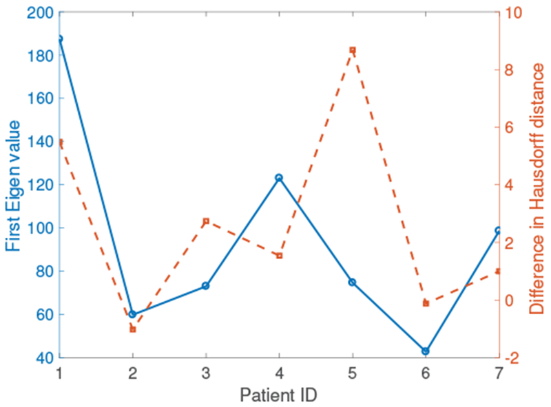
Results: A dataset of 7 subjects (4-7 scans) was collected and used to evaluate the proposed method by comparing its prediction Hausdorff distance errors against those of simple extrapolation. In addition, we evaluate the prediction results with respect to a conventional shape analysis technique such as Principal Component Analysis (PCA). All comparative results show the superior prediction performance of the proposed approach.

Conclusion: We introduce a novel approach to predict the AAA growth and its predicted uncertainty in future time, using longitudinal CT scans in a patient-specific fashion.

Significance: The capability to predict the AAA shape and its confidence region by our approach establish the potential for guiding clinicians with informed decision in conducting medical treatment and monitoring of AAAs.


Figures

Fig. 1.
Fig. 1.
Summary of our proposed method: point cloud data is inserted into the spatio-temporal Gaussian process regression as zero-value observations to generate the field. Then, the temporal evolution of the field is inferred through the dynamic model in (8). Finally, the AAA shape prediction and its uncertainty quantification are produced from the predicted field and the uncertainty field by utilizing the Kalman filter and the EM algorithm.
Fig. 2.
Fig. 2.
Example of an estimated field: cross section views of the 3D fielc at the same height in z-axis are shown at different times t. The on-surface points (where the field is zero) are labeled in white solid lines. The growth of the AAA in the radial direction can be visualized from top to bottom figures.
Fig. 3.
Fig. 3.
Convergence of the distance of (a) A and (b) σw to their equilibrium values (A and Σw∞), started with respect to different initial values of A and Σw.
Fig. 4.
Fig. 4.
The relative times of the scans compared to the first scan are plotted for each patient in days.
Fig. 5.
Fig. 5.
Fully trained case using all available longitudinal data: 3D rendering from the predicted (D^i,j) and true (Di,j) point clouds: The predicted and true point clouds are used to render the 3D surfaces using the Poisson reconstruction in Meshlab.
Fig. 6.
Fig. 6.
Uncertainty quantification for 7 patients for fully trained case: The implicit surfaces are regenerated on the grid by realizing the posteriori, multi-variate Gaussian distribution by (10). We then estimate the AAA surfaces that are corresponding to the realized implicit surfaces. Spatial regions that appear brighter means higher probability. The true cloud points are plotted in red dots.
Fig. 7.
Fig. 7.
Last-3 trained case using the most recent three longitudinal data points: 3D rendering from the estimated (D^i,j) and true (Di,j) point clouds: The predicted and true point clouds are used to render the 3D surfaces using the Poisson reconstruction in Meshlab. Note that we run the Last-3 trained case for patient P1, P2, P3, P4 and P6, since other cases already have 4 scans in total.
Fig. 8.
Fig. 8.
Uncertainty quantification for 5 patients for Last-3 trained case: The implicit surfaces are regenerated on the grid by realizing the multi-variate Gaussian distribution with the mean vector and covariance matrix computed in (5). Then, we estimate the AAA surfaces that are corresponding to the realized implicit surfaces. Each realization of the AAA surface from the posterior distribution is plotted with 2% occupancy. Therefore, spatial regions that appear brighter are more likely to be occupied by the AAA surface. The true cloud points are plotted in red dots. Note that we run the Last-3 trained case for patient P1, P2, P3, P4 and P6, since other cases already have 4 scans in total.
Fig. 9.
Fig. 9.
PCA for three particular patients P1, P4, and P6. Top to bottom: μ(x), μ(x) + σ1v1(x), and μ(x) + σ1v1(x), where μ(x), σ1, and v1(x) are the mean, first eigenvalue, and first eigenvector. From left to right: decreasingly ordered by the value of the first eigenvalue (maximum, medium, and minimum).
Fig. 10.
Fig. 10.
(a) Cumulative energy, global maximum diameter (in mm), and the volume of the AAA (in mm3) of 7 cases are shown in (a), (b), and (c), correspondingly.
Fig. 11.
Fig. 11.
The first eigenvalues (with the left scale) and the differences in the Hausdorff prediction errors (with the right scale) between the naive extrapolation and our method are shown over patient IDs in solid and dashed lines, respectively.
Fig. 12.
Fig. 12.
An example of usage of A(x) as an informative feature. Two successive shapes, namely previous and current shapes, are plotted in black squared and circled point clouds in standardized unit, respectively. Additionally, the intersections of them with the plane z = 0 are plotted in solid (previous) and dashed (current) white lines on the z = 0 plane. Furthermore, the cross-section views of the A(x) field at z = 0 and z = −1 are color plotted on the two planes. The migration of the surface is shown clearly in the direction indicated by the red arrow. Then, the velocity of the migration in the indicated direction can be computed by (11).

Similar articles

Cited by

References

    1. Porth CM, Essentials of pathophysiology: Concepts of altered health states. Lippincott Williams & Wilkins, 2010.
    1. Zankl AR, Schumacher H, Krumsdorf U, Katus HA, Jahn L et al., “Pathology, natural history and treatment of abdominal aortic aneurysms,” Clinical Research in Cardiology, vol. 96, no. 3, pp. 140–151, 2007. - PubMed
    1. Kent KC, “Abdominal aortic aneurysms,” New England Journal of Medicine, vol. 371, no. 22, pp. 2101–2108, 2014, pMID: [Online]. Available: 10.1056/NEJMcp1401430 - DOI - PubMed
    1. Klink A, Hyafil F, Rudd J, Faries P, Fuster V, Mallat Z, Meilhac O, Mulder WJ, Michel J-B, Ramirez F et al., “Diagnostic and thera-peutic strategies for small abdominal aortic aneurysms,” Nature Reviews Cardiology, vol. 8, no. 6, pp. 338–347, 2011. - PubMed
    1. Kniemeyer H, Kessler T, Reber PU, Ris HB, Hakki H, and Widmer MK, “Treatment of ruptured abdominal aortic aneurysm, a permanent challenge or a waste of resources? prediction of outcome using a multi-organ-dysfunction score,” European Journal of Vascular and Endovascular Surgery, pp. 190–196, 2000. - PubMed

Publication types