waveCSD: A method for estimating transmembrane currents originated from propagating neuronal activity in the neocortex: Application to study cortical spreading depression

Abstract

Background: Recent years have witnessed an upsurge in the development of methods for estimating current source densities (CSDs) in the neocortical tissue from their recorded local field potential (LFP) reflections using microelectrode arrays. Among these, methods utilizing linear arrays work under the assumption that CSDs vary as a function of cortical depth; whereas they are constant in the tangential direction, infinitely or in a confined cylinder. This assumption is violated in the analysis of neuronal activity propagating along the neocortical sheet, e.g. propagation of alpha waves or cortical spreading depression.

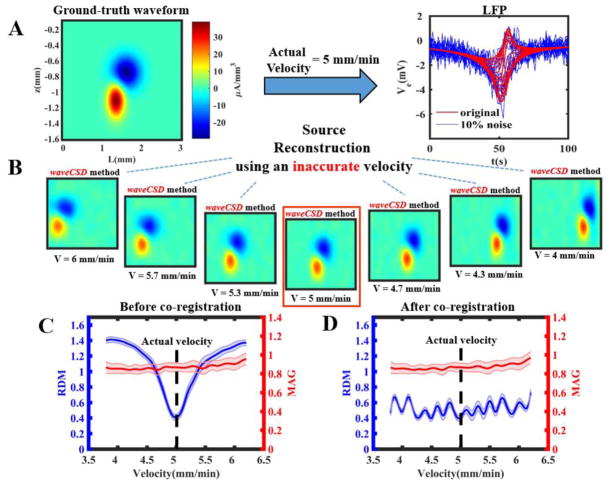
New method: Here, we developed a novel mathematical method (waveCSD) for CSD analysis of LFPs associated with a planar wave of neocortical neuronal activity propagating at a constant velocity towards a linear probe.

Results: Results show that the algorithm is robust to the presence of noise in LFP data and uncertainties in knowledge of propagation velocity. Also, results show high level of accuracy of the method in a wide range of electrode resolutions. Using in vivo experimental recordings from the rat neocortex, we employed waveCSD to characterize transmembrane currents associated with cortical spreading depressions.

Comparison with existing method(s): Simulation results indicate that waveCSD has a significantly higher reconstruction accuracy compared to the widely-used inverse CSD method (iCSD), and the regularized kernel CSD method (kCSD), in the analysis of CSDs originating from propagating neuronal activity.

Conclusions: The waveCSD method provides a theoretical platform for estimation of transmembrane currents from their LFPs in experimental paradigms involving wave propagation.

Keywords: Cortical spreading depression; Current source density analysis; Local field potential; Wave propagation.

Figure A1

Discretization of a rectangular grid of size n_x×n_y

Figure C1. Comparison of the accuracy of waveCSD, iCSD, and kCSD methods in the reconstruction of LFPs generated from a ground-truth waveform

A) A ground-truth waveform (the CSD profile, top left) is assumed to be generated 6 mm away from an A1x16 probe, inserted perpendicularly in the cortex with an inter-electrode spacing of 100 μm. The first electrode is assumed to be 100 μm deep in the brain tissue. Here, the waveform propagates towards the electrodes at a constant velocity of 4 mm/min. The resultant LFPs are shown in the top right panel (black → most superficial electrode, and red → deepest electrode in the probe). B) Model parameter estimation for kCSD method using k-fold cross-validation technique as described in (Potworowski et al., 2012). The left panel shows cross-validation error for a wide range of R and h values, and the inset confirms that the selected parameters (the red dot) coincide with the global minimum of cross-validation error values. The estimated diameter (2R) for the kCSD method is used for source reconstruction in the iCSD method shown in panel C. C) Source reconstruction using iCSD, kCSD and waveCSD methods without the presence of noise in the LFP data. (iCSD- RDM: 0.62, MAG: 0.18; kCSD- 0.62, MAG: 0.33, waveCSD- RDM: 0.01, MAG: 0.99). Both RDM and MAG measures confirm that the waveCSD method provides more accurate CSD reconstruction among all methods (i.e. RDM closer to zero and MAG closer to 1 in the waveCSD method). For better visualization, colorbar ranges are different in figures. Parameters: waveCSD method- same as Fig. 1. kCSD method- R = 1.6 [mm]; h = 0.14. D) mean±std for RDM and MAG of 50 realization of the noisy LFP data at each noise level for all three methods. Noise reduction in the iCSD method was performed by applying a Gaussian spatial filter on the reconstructed CSD from unfiltered LFP recordings (Gaussian filter sigma: σ_gf = 0.1 [mm]).

Figure C2. Comparison of the accuracy of waveCSD, iCSD, and kCSD methods in the reconstruction of LFPs generated from a ground-truth waveform

A) A ground-truth waveform (the CSD profile, top left) is assumed to be generated 6 mm away from an A1x16 probe, inserted perpendicularly in the cortex with an inter-electrode spacing of 100 μm. The first electrode is assumed to be 100 μm deep in the brain tissue. Here, the waveform propagates towards the electrodes at a constant velocity of 4 mm/min. The waveform is generated by superposition of 10 random Gaussian sources with random amplitude, spread, and angles. The resultant LFPs are shown in the top right panel (black → most superficial electrode, and red → deepest electrode in the probe). B) Model parameter estimation for kCSD method using k-fold cross-validation technique as described in (Potworowski et al., 2012). The left panel shows cross-validation error for a wide range of R and h values, and the inset confirms that the selected parameters (the red dot) coincide with the global minimum of cross-validation error values. The estimated diameter (2R) for the kCSD method is used for source reconstruction in the iCSD method shown in panel C. C) Source reconstruction using iCSD, kCSD and waveCSD methods without the presence of noise in the LFP data. For comparison purposes, colorbar ranges and labels are the same as in C1 A left panel. (iCSD- RDM: 0.64, MAG: 0.54; kCSD- 0.66, MAG: 0.72, waveCSD-RDM: 0.05, MAG: 0.99). Both RDM and MAG measures confirm that the waveCSD method provides more accurate CSD reconstruction among all methods (i.e. RDM closer to zero and MAG closer to 1 in the waveCSD method). Parameters: waveCSD method- same as Fig. 1. kCSD method- R = 2.2 [mm]; h = 0.35. D) mean±std for RDM and MAG of 50 realization of the noisy LFP data at each noise level for all three methods. Noise reduction in the iCSD method was performed by applying a Gaussian spatial filter on the reconstructed CSD from unfiltered LFP recordings (Gaussian filter sigma: σ_gf = 0.1 [mm]).

Figure 1. Comparison of the accuracy of waveCSD, iCSD, and kCSD methods in the reconstruction of LFPs generated from a ground-truth waveform

A) A ground-truth waveform (the CSD profile, top left) is assumed to be generated 6 mm away from an A1x16 probe, inserted perpendicularly in the cortex with an inter-electrode spacing of 100 μm. The first electrode is assumed to be 100 μm deep in the brain tissue. Here, the waveform propagates towards the electrodes at a constant velocity of 4 mm/min. The resultant LFPs are shown in the top right panel (black → most superficial electrode, and red → deepest electrode in the probe). B) Model parameter estimation for kCSD method using k-fold cross-validation technique as described in (Potworowski et al., 2012). The left panel shows cross-validation error for a wide range of R and h values, and the inset confirms that the selected parameters (the red dot) coincide with the global minimum of cross-validation error values. The estimated diameter (2R) for the kCSD method is used for source reconstruction in the iCSD method shown in panel C. C) Source reconstruction using iCSD, kCSD and waveCSD methods without the presence of noise in the LFP data. (iCSD- RDM: 0.47, MAG: 0.67; kCSD- 0.47, MAG: 0.88, waveCSD- RDM: 0.01, MAG: 0.99). Both RDM and MAG measures confirm that the waveCSD method provides more accurate CSD reconstruction among all methods (i.e. RDM closer to zero and MAG closer to 1 in the waveCSD method). For comparison purposes, colorbar ranges and labels are the same as in 1 A left panel. Parameters: waveCSD method- The temporal resolution of the Q matrix is 1 [s]. n_τ = 40; n_z = 30; L = 3 [mm]; σ = 0.3 [S/mm]; α = 3.5 [mm]. kCSD method- R = 2.2 [mm]; h = 0.44 [mm]; number of sources (nSrc) = 320. iCSD method- d = 4.4 [mm].

Figure 2. Effect of observation noise on reconstruction accuracy of waveCSD compared to iCSD and kCSD

Accuracy of reconstruction of all methods are compared for different values of Gaussian observation noise (as percent of the maximum LFP signal) added to the LFP data shown in Fig. 1, top right panel. A) RDM values for all three methods across 50 realizations of the observations are shown as mean±std for each noise level. Noise reduction in the iCSD method was performed by applying a Gaussian spatial filter on the reconstructed CSD from unfiltered LFP recordings (Gaussian filter sigma: σ_gf = 0.1 [mm]) Results indicate that at all noise levels waveCSD method outperforms iCSD and kCSD methods (RDM values closer to zero in waveCSD). B) MAG values for all three methods across 50 realizations of the observations are shown as mean±std for each noise level. Results show a decreasing trend in the MAG measure for waveCSD method as the noise level increases, while both iCSD and kCSD methods show the opposite trend. Two examples of the average reconstructed CSD profile using all three methods are provided in panels C and D for 10 and 30% noise levels, respectively. Parameters are as stated in Fig. 1.

Figure 3. Effect of waveform velocity on the reconstruction accuracy of waveCSD, kCSD and iCSD methods

The accuracy of methods, as measured by RDM and MAG, are compared as a function of the known velocity of the ground-truth waveform presented in Figure 1A, top left panel. 10% Gaussian noise was added to the LFP data, and optimal parameters of kCSD and iCSD methods were selected for each velocity value as explained in section 2.3. RDM and MAG values are shown as mean±std across 50 realizations of the observation noise. Noise reduction in the iCSD method was performed by applying a Gaussian spatial filter on the reconstructed CSD from unfiltered LFP recordings (Gaussian filter sigma: σ_gf = 0.1 [mm]). A) kCSD and iCSD show no change in the RDM value at different velocities, while waveCSD RDM increases slightly with the increase in wave velocity. B) All MAG traces remain almost unchanged across different velocity values. Two examples of the average reconstructed CSD profile using all three methods are provided in panels C and D for 3 and 7 mm/min wave velocity, respectively. Parameters are as stated in Fig. 1.

Figure 4. Dependency of CSD reconstruction accuracy to the diameter of the designated cylinder used in the iCSD method

The top panel shows that both RDM and MAG values in the iCSD method decrease as a function of d. However, the changes are more drastic for the MAG measure (MAG: ~4.5 → ~1.5; RDM: ~0.85 → ~0.75, for d: 300 →700 μm). A limit case of d → ∞ is also provided in the bottom panel. Noise reduction in the iCSD method was performed by applying a Gaussian spatial filter on the reconstructed CSD from unfiltered LFP recordings (Gaussian filter sigma: σ_gf = 0.1 [mm]). waveCSD method is independent of d, thereby both measures are constant throughout. v = 4 mm/min, and 10% noise is added to the LFP data. The rest of the parameters are as stated in Fig. 1.

Figure 5. Robustness of the CSD analysis using waveCSD method to noise and electrode resolution

A–B) RDM and MAG measures are shown for c_waveCSD from the LFP data in Fig. 1A right panel, for a range of known velocities and different noise levels. The colorbar for the MAG measure is inverted compared to RDM (blue colored regions indicate desirable RDM and MAG values; red regions indicate areas with high error in reconstruction). At any given velocity, increase in the noise level decreases the accuracy of the reconstruction (RDM away from zero, and MAG away from one) and vice versa. C–D) RDM and MAG measures are shown as a function of electrode resolution at different noise levels for the average reconstructed CSD profile (c_waveCSD) of the LFP data of the ground-truth waveform. At any electrode resolution, increase in the noise level decreases the accuracy of reconstruction, whereas at any given noise, increasing the number of recording electrodes, increases the reconstruction accuracy. Parameters are as described in Fig. 1 except n_τ = 30 and n_z = 10.

Figure 6. Reconstruction accuracy under uncertainties in the knowledge of velocity of the waveform in the waveCSD method

A) Under 10% noise, LFPs (right panel, red traces: unnoisy, blue traces: noisy) from an A1x16 probe were simulated assuming a ground-truth CSD waveform (left panel) propagating with at v = 5 mm/min towards the electrodes. B) The noisy simulated LFPs were used to estimate the CSD using the waveCSD method assuming a range of wave velocities from 4 to 6 mm/min. Profiles show a monotonic shift in the position of CSDs relative to the error in the assumed velocity. C) RDM and MAG measures for the reconstructed profiles using velocity values are shown as mean±std. If the actual velocity is used for the reconstruction (highlighted box in panel B), the accuracy is maximal. Note that the RDM measure is significantly dependent on the velocity error, while the MAG measure does not significantly change. D) Both RDM and MAG are almost unchanged after linear coregistration of reconstructed profiles in panel B along the x axis. Parameters used in simulations: temporal resolution of the Q matrices: 1 [s]; n_τ = 20; n_z = 10. Rest of the parameters are as described in Fig. 1.

Figure 7. waveCSD model parameter estimation from the LFP data using GCV technique

A) A ground-truth profile was generated via superposition of 10 Gaussian profiles with random amplitude, spread, and angle (left panel). The resultant LFP profile (right panel) were generated from a A1x16 electrode assuming the waveform was generated 6 mm away from the electrodes and propagated towards the probe with a velocity of 5 mm/min (black → most superficial electrode, and red → deepest electrode in the probe). The limits of the cortex in the y direction (i.e. Y_f =−y_s = α) was set to be from [-3, 3] [mm]. B) For a wide range of velocity and α values the corresponding Q matrices were calculated (blue dots) and the parameter pair which minimized the GCV score was selected as the optimal set (the red dot). RDM and MAG measures are also shown for each parameter pair. In all simulations in the panel no noise was added to the LFP data. C) Parameter estimation was performed in the presence of varying percentages of the observation noise in the LFP data. For each noise level and each parameter set, 50 realizations of the noisy data were reconstructed. Data is shown is mean±std, and the actual values of velocity and α are shown in red dashed lines.

Figure 8. CSD analysis of LFPs recorded during cortical spreading depression in rats using the waveCSD method

A) The LFP recordings of one rat using an A1x32 probe during cortical spreading depression is shown in the left panel. The resting brain activity and silencing period after the event were excluded in the source reconstruction using the waveCSD method (right panel). LFP data was resampled to the temporal resolution of the Q matrix used for the CSD analysis (i.e., 0.2 [s]). The resampled data is shown using a color gradient from black to red (black → most superficial electrode, and red → deepest electrode in the probe). B) Reconstructed CSD profile of the resampled LFP data in panel A inset using the waveCSD method. C) Heat maps of the resampled LFP and the simulated LFP (resulting from forward modeling of the profile in the panel B using Eq. (8)) are demonstrated. Please note that panels B and C have different x-axes. For the reconstructed waveCSD model (panel B), the x-axis represents space, along the propagating direction. For the LFP heat maps (panel C), the x-axis represents time. D) Simulated LFP is superimposed onto the original resampled LFP. The insets demonstrate the electrodes with the best and the worst reconstruction determined based on the sum of square of the errors between the original and the reconstructed trace. Parameters used for the computation of the Q matrix for CSD analysis of the data: n_τ = 30; n_z = 20; L = 1 [mm]; temporal resolutions: 0.2 [s]. The rest of parameters are as described in Fig. 1.

Figure 9. Average profile of transmembrane current sources during cortical spreading depression in rats after nonlinear coregistration of the reconstructed profiles

A) The grand average transmembrane CSD profile across five rats during cortical spreading depression using the waveCSD method is depicted. The averaging was performed after application of a landmark-based nonlinear diffeomorphic coregistration to individual reconstructed current sources. B) The histology image showing the accurate positioning and the desired penetration depth of the probe in the rat neocortex. C) The schematic representing major cellular substrates across different layers (i.e., Supra-Granular, Granular, and Infra-Granular) of the rat neocortex, e.g. excitatory pyramidal cells (layer II/III – black, layer V – brown and layer VI – blue), excitatory spiny stellate cells (yellow), inhibitory interneurons (basket cells – blue/black and Martinotti cells – red/blue), and layer II/III glia cells (green).

References

1. Aroniadou VA, Keller A. The patterns and synaptic properties of horizontal intracortical connections in the rat motor cortex. Journal of neurophysiology. 1993;70:1553–69. - PubMed
1. Barth DS, Baumgartner C, Di S. Laminar interactions in rat motor cortex during cyclical excitability changes of the penicillin focus. Brain research. 1990;508:105–17. - PubMed
1. Basarsky TA, Duffy SN, Andrew RD, MacVicar BA. Imaging spreading depression and associated intracellular calcium waves in brain slices. Journal of Neuroscience. 1998;18:7189–99. - PMC - PubMed
1. Berens P, Keliris GA, Ecker AS, Logothetis NK, Tolias AS. Feature selectivity of the gamma-band of the local field potential in primate primary visual cortex. Frontiers in neuroscience. 2008;2:199. - PMC - PubMed
1. Box GE, Cox DR. An analysis of transformations. Journal of the Royal Statistical Society. Series B (Methodological) 1964:211–52.
Publication types
LinkOut - more resources