Valid molecular dynamics simulations of human hemoglobin require a surprisingly large box size

Abstract

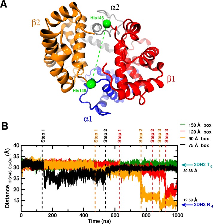
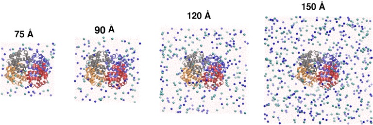
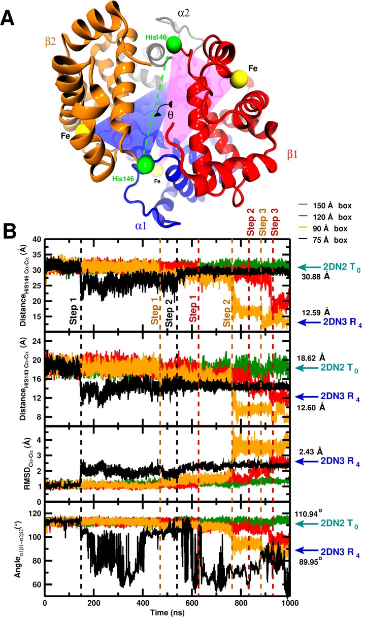
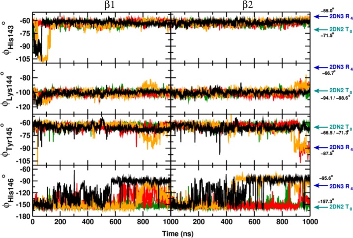
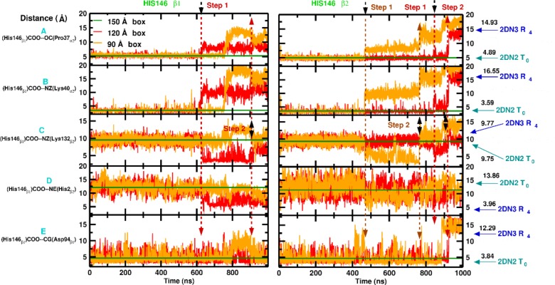
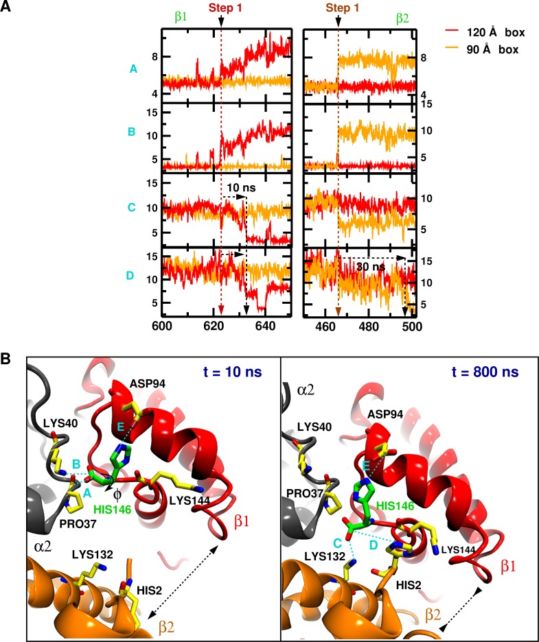
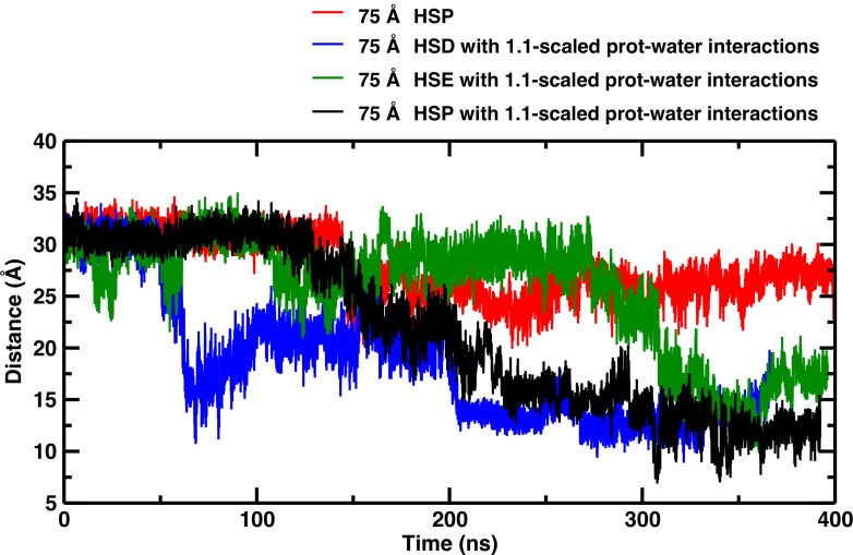
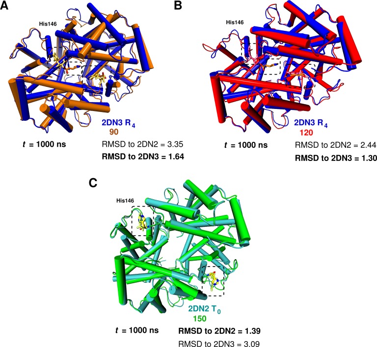
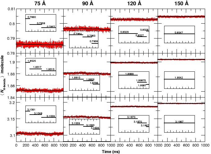
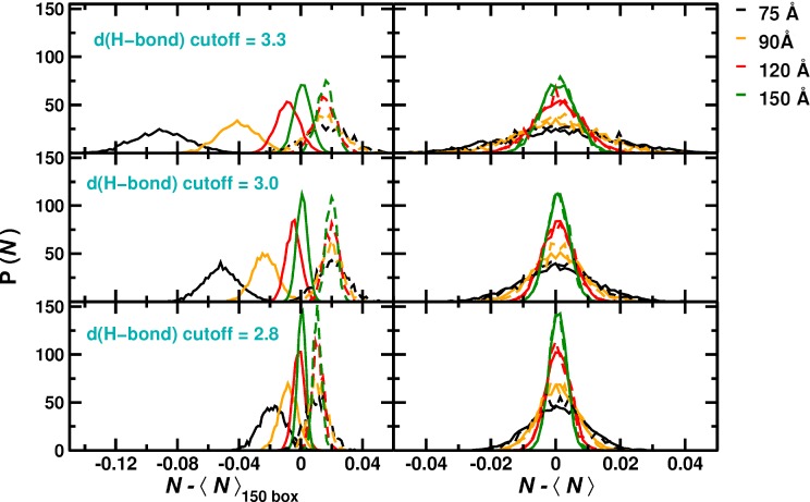
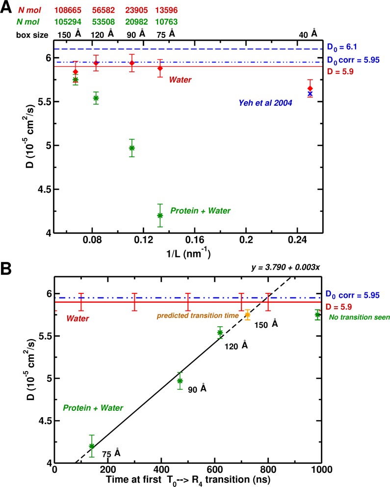
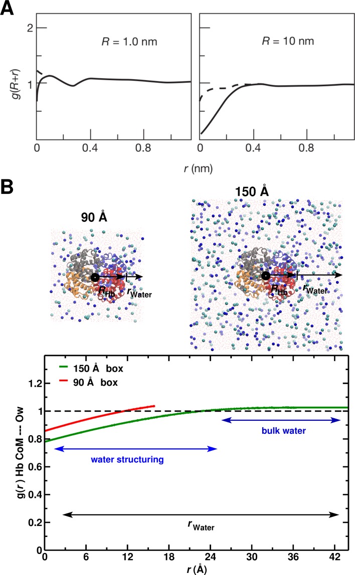
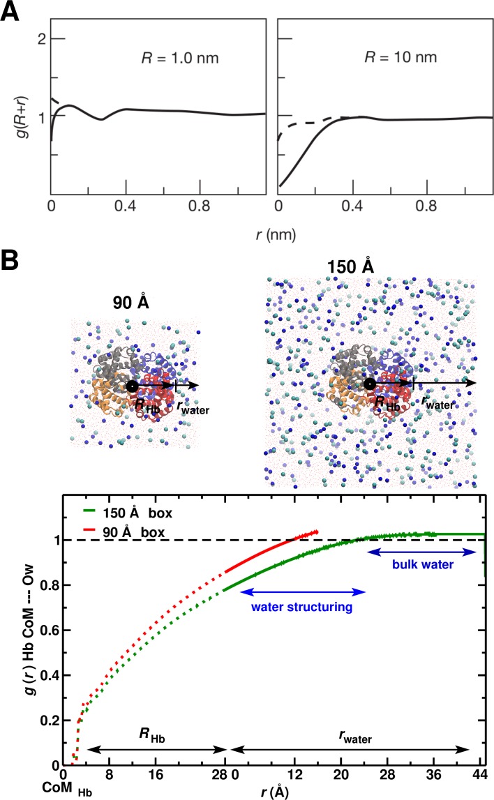
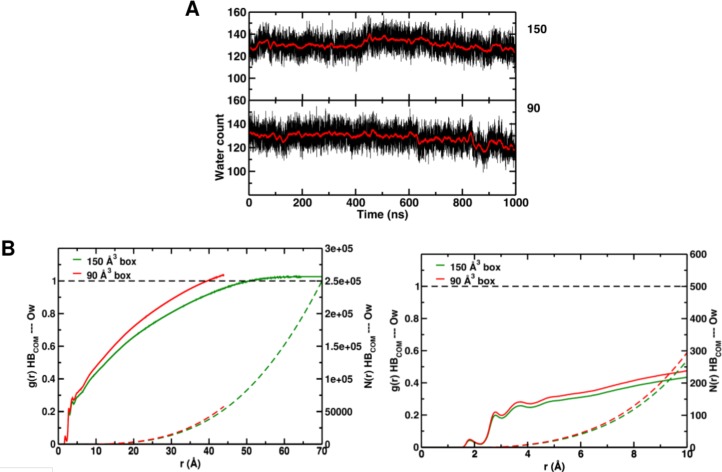
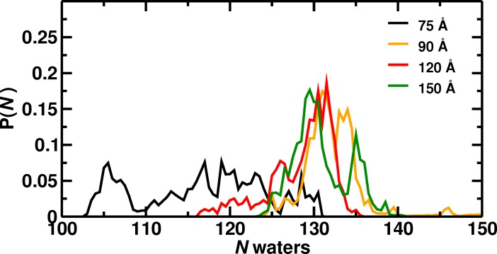
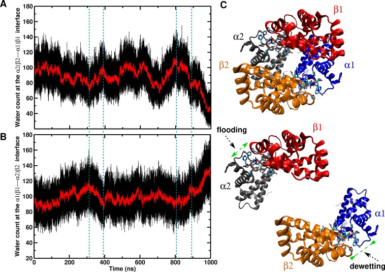
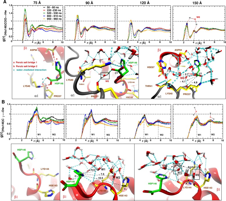
Recent molecular dynamics (MD) simulations of human hemoglobin (Hb) give results in disagreement with experiment. Although it is known that the unliganded (T[Formula: see text]) and liganded (R[Formula: see text]) tetramers are stable in solution, the published MD simulations of T[Formula: see text] undergo a rapid quaternary transition to an R-like structure. We show that T[Formula: see text] is stable only when the periodic solvent box contains ten times more water molecules than the standard size for such simulations. The results suggest that such a large box is required for the hydrophobic effect, which stabilizes the T[Formula: see text] tetramer, to be manifested. Even in the largest box, T[Formula: see text] is not stable unless His146 is protonated, providing an atomistic validation of the Perutz model. The possibility that extra large boxes are required to obtain meaningful results will have to be considered in evaluating existing and future simulations of a wide range of systems.

Keywords: diffusion constant; hemoglobin; hydrophobic effect; molecular biophysics; molecular dynamics; none; simulation box size; structural biology.

Figure 1.. Global structural changes depending on box size.

Panel A: Overall structure of the $\alpha 1\beta 1\alpha 2\beta 2$ hemoglobin tetramer. The His146 side chains (green spheres) are specifically indicated. Panel B: Temporal change of the C$\alpha$–C$\alpha$ distance between His146${}_{\beta 1}$ and His146${}_{\beta 2}$. The dashed lines (black, orange, red) indicate transition points for the 75, 90, and 120 box, respectively. Cyan and blue arrows indicate the values of the corresponding observable found for the deoxy T${}_0$ (2DN2) and oxy R${}_4$ (2DN3) states, respectively.

Figure 1—figure supplement 1.. Tetrameric hemoglobin solvated in boxes of different sizes.

Tetrameric hemoglobin solvated in boxes of size: (from left to right) 75, 90, 120 and 150 Å. Spheres correspond to Na${}^{+}$ and Cl${}^{-}$ ions, added to neutralize the system and to achieve a biologically appropriate salt concentration of 0.15 mol/L.

Figure 1—figure supplement 2.. Global structural changes depending on box size.

Panel A: Overall structure of the $\alpha 1\beta 1\alpha 2\beta 2$ hemoglobin tetramer. The iron atoms (Fe, yellow spheres) and His146 side chains (green spheres) are specifically indicated. The angle $\theta$ measures the angle between the two planes containing His146${}_{\beta 1}$Fe${}_{\beta 1}$Fe${}_{\alpha 1}$ and His146${}_{\beta 2}$Fe${}_{\beta 2}$Fe${}_{\alpha 2}$, respectively. Panel B: temporal change of (from top to bottom) the C$\alpha$–C$\alpha$ distance between His146${}_{\beta 1}$ and His146${}_{\beta 2}$, the C$\alpha$–C$\alpha$ distance between His143${}_{\beta 1}$ and His143${}_{\beta 2}$, C$\alpha$ RMSD relative to the 2DN2 X-ray structure, and the angle $\theta$. The dashed lines (black, orange, red) indicate transition points for the 75, 90, and 120 Å boxes, respectively. Cyan and blue arrows indicate the values of the corresponding observables found for the deoxy T${}_0$ (2DN2) and oxy R${}_4$ (2DN3) states, respectively. Top panel is also given in the main MS.

Figure 1—figure supplement 3.. Local structural rearrangement of the C-terminus of the β chain.

From top to bottom: the Ramachandran $\varphi$-angle of His143, Lys144, Tyr145 and His146. Left panels report time series for $\beta 1$, and right panels those for $\beta 2$. Cyan and blue arrows indicate the corresponding values found in crystal structure of the deoxy (2DN2) and oxy (2DN3) state, respectively. Color code as in Figure 1—figure supplement 1.

Figure 1—figure supplement 4.. Local structural changes around His146.

Left: Interactions involving His146${}_{\beta }$. Right: Interactions involving His146${}_{\beta }$. From top to bottom: [a] water-mediated contact between (His146${}_{\beta }$)COO${}^{-}$–OC(Pro37${}_{\alpha }$), [b] the salt bridge between (His146${}_{\beta }$)COO${}^{-}$–NZ(Lys40${}_{\alpha }$), [c] the contact between (His146${}_{\beta }$)COO${}^{-}$–NZ(Lys132${}_{\beta }$), [d] the contact between (His146${}_{\beta }$)COO${}^{-}$ and NE(His2${}_{\beta }$) and [e] the salt bridge between (His146${}_{\beta }$)NE2 and COO${}^{-}$(Asp94${}_{\beta }$). Cyan and blue arrows indicate the corresponding values found in crystal structure of the deoxy (2DN2) and oxy (2DN3) state, respectively. The dashed lines indicate breaking points along the 1$\mu$s MD simulation and the black arrows indicates the first to break. The straight green line represents the averaged distance over 1 $\mu$s of MD simulation for the 150 Å box as reference.

Figure 1—figure supplement 5.. Structural transition details.

(A) Close-up of the [600;650] and [440;520] ns interval of Figure 1—figure supplement 1, illustrating the order of events for transitions in the 120 (left panel) and 90 Å box (right panel), respectively. Black arrows indicates the transmission of the structural modifications. (B) Structural details for every quantity from the 90 Å box at 10 and 800 ns, respectively. The dashed black arrow indicates the separation distance between $\beta 1$ and $\beta 2$.

Figure 1—figure supplement 6.. Temporal structural changes of the Cα–Cα distance between His146β1 and His146β2 in the 75 Å box for different simulation conditions.

Temporal structural changes of the C$\alpha$–C$\alpha$ distance between His146${}_{\beta 1}$ and His146${}_{\beta 2}$, depending on the protonation state of His 146 in the 75 Å box with and without scaled protein-water interactions.

Figure 2.. Global conformational rearrangement of tetrameric hemoglobin as a function of the box size.

(A) Superposition of the 2DN3 structure and the Hb structure in the 90 Å box at $t=1000$ ns. (B) Superposition of the 2DN3 structure and the Hb structure in the 120 Å box at $t=1000$ ns. (C) Superposition of the 2DN2 structure and the structure in the 150 Å box at $t=1000$ ns. In each case the RMSDs (in Å) to the 2DN2 and 2DN3 are also given.

Figure 3.. The average number of H-bonds per water molecule <NH−bonds>/molecule, from analyzing water-water hydrogen bonds, during 1 μs MD simulations for all four box sizes and for three different donor-acceptor distance cutoffs: 2.8 (strong, top panels), 3.0 (medium, middle panels) and 3.3 Å (weak, bottom panels).

The solid black lines are averages for time intervals corresponding to the lifetime of each state in each of the simulation boxes (see Figure 1): For the 75 Å box: 0 to 140 ns (first transition), 140 to 530 ns (second transition) and 530 to 1000 ns. For the 90 Å box: 0 to 470 ns, 470 to 780 ns and 780 to 1000 ns. For the 120 Å box: 0 to 620 ns, 620 to 920 ns, and 920 to 1000 ns. For the 150 Å box, the average is over the entire simulation since no transition occurs. The average reduction in $<N_{\text{H}-\text{bonds}}>$/molecule is maximum (0.1) when weak H-bonds are included (cutoff 3.3 Å, bottom row) and smallest (0.015) if only strong H-bonds (cutoff 2.8 Å, top row) are analyzed. In the 120 Å box (third column) and for the strong H-bonds the loss in $<N_{\text{H}-\text{bonds}}>$/molecule is insignificant but clearly increases when weak H-bonds are included. We also observe a significant decrease in the fluctuation of $<N_{\text{H}-\text{bonds}}>$/molecule between simulations in the smallest and the largest box sizes and a pronounced drop in $<N_{\text{H}-\text{bonds}}>$/molecule for the 75 and 90 Å boxes prior to the transitions, see insets.

Figure 3—figure supplement 1.. Number N of H-bonds and their fluctuations δN for pure water and simulations including the protein for the four box sizes.

Left column: Probability distribution of number of H-bonds $N$ relative to the average of the 150 Å box. Right column: probability distribution of the fluctuation $\delta N$ for each box individually. The left column illustrates the loss in the average number of $N$ relative to the 150 Å box for smaller box sizes. This loss increases with including medium ($d=3.0$ Å) and weak ($d=3.3$ Å) H-bonds. Solid lines for simulations including the protein, broken lines for pure water boxes. As can be seen (left column), for a box size of 150 Å (solid and broken green lines) the average number of Hbonds with and without protein changes only marginally, whereas for a 75 Å box these numbers (solid and broken black lines) differ considerably. Also, the $\delta N$ depends sensitively on the box size.

Figure 4.. System-size dependence of the water diffusion coefficient.

(A) Water diffusion coefficients $D$ as a function of system size for systems with and without protein. Also, results from Hummer et al. are shown for comparison and validation. (B) The water $D$ as a function of time for the first instability to occur. For the 75, 90, and 120 Å boxes instabilities were observed (see Figure 1) and scale linearly with the water $D$. The yellow symbol for the 150 Å box is the extrapolated value (700 ns).

Figure 5.. System-size dependence of the average equilibrium water density.

(A) From Ref. (Chandler, 2005) (Figure 3); the average equilibrium water density a distance $r+R$ from spherical cavities. $R$ is the (spherical) size of the solute. Solid lines for the ideal hydrophobe, dashed line when van der Waals interactions are present. (B) Results for Hb in water for the 90 Å (red) and 150 Å (green) box. The radius of Hb (2.8 nm) is intermediate between the two cases in panel A.

Figure 5—figure supplement 1.. Enhanced version of Figure 5 from the main MS.

A: From Ref.(Chandler, 2005) (Figure 3); the average equilibrium water density a distance $r+R$ from spherical cavities. $R$ is the (spherical) size of the solute and $r$ is the distance from the surface of the hydrophobe. Solid lines for the ideal hydrophobe, dashed line when van der Waals interactions are present. The radial distribution function reaches the bulk value $\sim 25$ Å away from the solute’s surface. B: results for Hb in water for the 90 Å (red) and 150 Å (green) box. The radius of Hb (2.8 nm or 28 Å) is intermediate between the two cases in panel A. The $r-$coordinate is split in two segments the first (running from 0 to 28 Å) is the region inside Hb. The second (from 0 to 45 Å) is the region outside Hb. The radial distribution function reaches the bulk value $\sim 20$ Å away from the solute’s surface.

Figure 5—figure supplement 2.. Number of water molecules in the central cylinder of Hb.

Panel A: Time series for the number of water molecules in the central cylinder (see also Figure 5—figure supplement 3) for 90 Å and 150 Å boxes. Panel B: radial distribution function $g\left(r\right)$ (solid lines) and $N\left(r\right)$ (dashed lines) for 90 and 150 Å boxes. The left panel shows the entire range $r$ of distances from the center of the protein and the right panel only that concerning the central cylinder. The value of $N(r=8.5)$ is 150 which is consistent with the results from explicit counting and confirms that the $g\left(r\right)$ is meaningful.

Figure 5—figure supplement 3.. Distribution P(N) of water molecules in the central cylinder for the different box sizes.

Probability distribution of the number of water molecules inside Hb over 1 $\mu$s of MD simulation depending on box size. The water count includes only waters in the central cylinder and not waters at the tetramerization interface. The region was defined as a cylinder of 8.5 Å radius and 22 Å of height and having as center the center of mass of the 4 Heme moieties.

Figure 5—figure supplement 4.. Water at the (α1β2):(α2β1) interface.

The number of water molecules at the $\left(\alpha 1\beta 2\right):\left(\alpha 2\beta 1\right)$ interface from 1 $\mu$s MD for the 90 Å box. (A) Time series of the $\beta 1:\alpha 2$ interface. (B) Time series of the $\beta 2:\alpha 1$ interface. (C) Illustration of the studied regions. The transitions occur at 480, 780 and 880 ns, respectively.

Figure 6.. Averaged radial distribution functions g(r) between His146 and water for the different box sizes and for simulation windows before, during and after the structural transitions (see Figure 1).

Analysis for (A) the C-terminal (CT) of His146 and Water H (Hw) and (B) for C of His146 and water O (Ow). For the largest (150 Å) box no appreciable change in $g\left(r\right)$ is found. The two peaks at 2.7 and 4.1 Å in (A) and the two peaks at 5 and 7.5 Å in (B) are due to a water network as indicated in the sketches. The sketches in A and B represent different views of the same snapshot taken from the MD simulation of the 150 Å box at $t=960$ ns and is used here as reference to describe the water network because this box represented a stable $g\left(r\right)$. Sketches in (A) emphasise the water network at the C-terminal of His146, and sketches in (B) emphasise the water network at the C${}_{\gamma }$ of His146. Waters W0, W1 and W2 are key structural waters (used as anchor) in the stability of the T state (they are framed with a black line). This network is stable for simulations in the largest box but unstable in the other boxes. His143 is singly protonated (${\displaystyle \mathrm{N}ϵ}$) and His146 is doubly protonated (N$\delta$ and N$ϵ$).

References

1. Abraham MJ, Murtola T, Schulz R, Páll S, Smith JC, Hess B, Lindahl E. GROMACS: high performance molecular simulations through multi-level parallelism from laptops to supercomputers. SoftwareX. 2015;1-2:19–25. doi: 10.1016/j.softx.2015.06.001. - DOI
1. Allen MP, Tildesley DJ. Computer Simulation of Liquids. Oxford, U.K: Clarendon Press; 1987.
1. Baldwin J, Chothia C. Haemoglobin: the structural changes related to ligand binding and its allosteric mechanism. Journal of Molecular Biology. 1979;129:175–220. doi: 10.1016/0022-2836(79)90277-8. - DOI - PubMed
1. Best RB, Zheng W, Mittal J. Balanced Protein-Water interactions improve properties of disordered proteins and Non-Specific protein association. Journal of Chemical Theory and Computation. 2014;10:5113–5124. doi: 10.1021/ct500569b. - DOI - PMC - PubMed
1. Best RB, Zhu X, Shim J, Lopes PE, Mittal J, Feig M, Mackerell AD. Optimization of the additive CHARMM all-atom protein force field targeting improved sampling of the backbone φ, ψ and side-chain χ(1) and χ(2) dihedral angles. Journal of Chemical Theory and Computation. 2012;8:3257–3273. doi: 10.1021/ct300400x. - DOI - PMC - PubMed
Publication types