

A Comparative Study of Four Kinds of Adaptive Decomposition Algorithms and Their Applications
- PMID: 30004429
- PMCID: PMC6068995
- DOI: 10.3390/s18072120
A Comparative Study of Four Kinds of Adaptive Decomposition Algorithms and Their Applications
Abstract
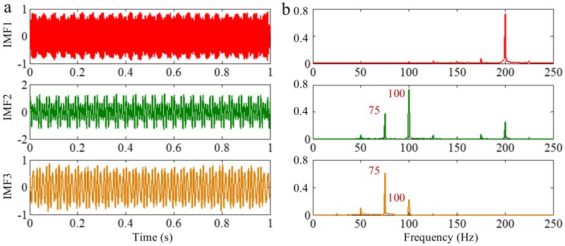
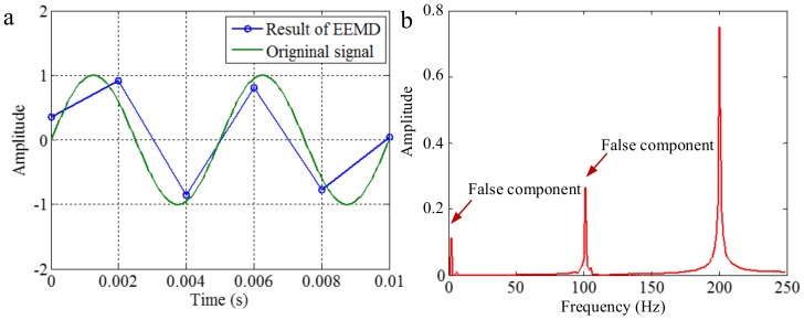
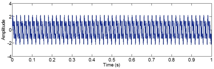
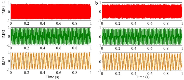
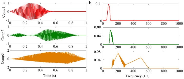
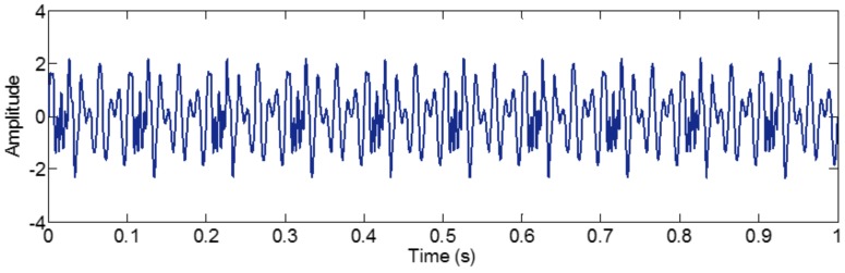
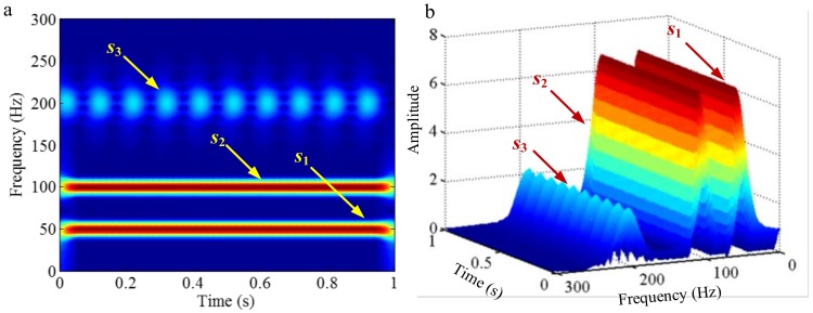
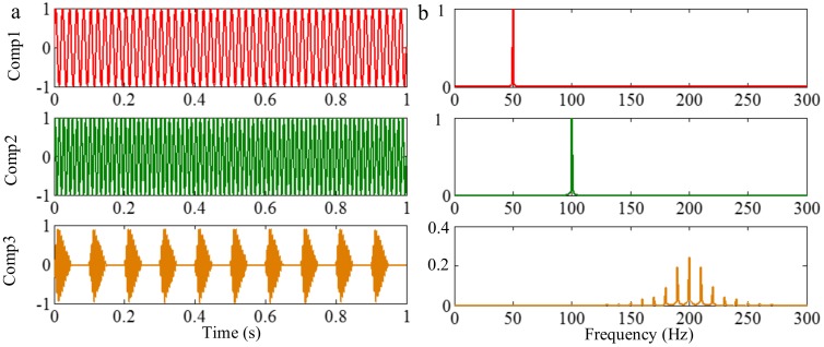
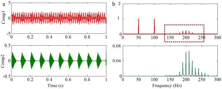
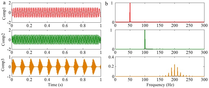
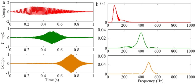
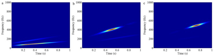
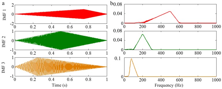
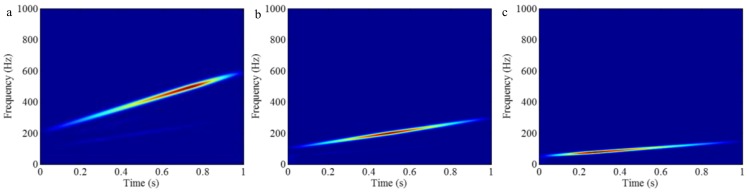
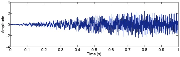
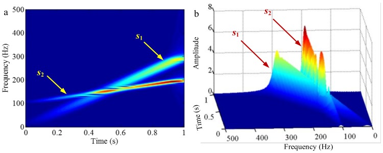
The adaptive decomposition algorithm is a powerful tool for signal analysis, because it can decompose signals into several narrow-band components, which is advantageous to quantitatively evaluate signal characteristics. In this paper, we present a comparative study of four kinds of adaptive decomposition algorithms, including some algorithms deriving from empirical mode decomposition (EMD), empirical wavelet transform (EWT), variational mode decomposition (VMD) and Vold⁻Kalman filter order tracking (VKF_OT). Their principles, advantages and disadvantages, and improvements and applications to signal analyses in dynamic analysis of mechanical system and machinery fault diagnosis are showed. Examples are provided to illustrate important influence performance factors and improvements of these algorithms. Finally, we summarize applicable scopes, inapplicable scopes and some further works of these methods in respect of precise filters and rough filters. It is hoped that the paper can provide a valuable reference for application and improvement of these methods in signal processing.
Keywords: adaptive decomposition algorithm; narrow-band signal; non-stationary signal; signal processing.
Conflict of interest statement
The authors declare no conflicts of interest.
Figures

Similar articles
-
A Novel Adaptive Signal Processing Method Based on Enhanced Empirical Wavelet Transform Technology.Sensors (Basel). 2018 Oct 3;18(10):3323. doi: 10.3390/s18103323. Sensors (Basel). 2018. PMID: 30282951 Free PMC article.
-
Wavelet transform-based mode decomposition for EEG signals under general anesthesia.PeerJ. 2024 Nov 15;12:e18518. doi: 10.7717/peerj.18518. eCollection 2024. PeerJ. 2024. PMID: 39559333 Free PMC article.
-
Multimode Decomposition and Wavelet Threshold Denoising of Mold Level Based on Mutual Information Entropy.Entropy (Basel). 2019 Feb 21;21(2):202. doi: 10.3390/e21020202. Entropy (Basel). 2019. PMID: 33266917 Free PMC article.
-
A Comparative Analysis of Signal Decomposition Techniques for Structural Health Monitoring on an Experimental Benchmark.Sensors (Basel). 2021 Mar 5;21(5):1825. doi: 10.3390/s21051825. Sensors (Basel). 2021. PMID: 33807884 Free PMC article. Review.
-
Resonance-Based Sparse Signal Decomposition and its Application in Mechanical Fault Diagnosis: A Review.Sensors (Basel). 2017 Jun 3;17(6):1279. doi: 10.3390/s17061279. Sensors (Basel). 2017. PMID: 28587198 Free PMC article. Review.
Cited by
-
Application of EEG in migraine.Front Hum Neurosci. 2023 Feb 17;17:1082317. doi: 10.3389/fnhum.2023.1082317. eCollection 2023. Front Hum Neurosci. 2023. PMID: 36875229 Free PMC article. Review.
-
Matrix Pencil Method for Vital Sign Detection from Signals Acquired by Microwave Sensors.Sensors (Basel). 2021 Aug 26;21(17):5735. doi: 10.3390/s21175735. Sensors (Basel). 2021. PMID: 34502626 Free PMC article.
-
A genetic algorithm optimized hybrid model for agricultural price forecasting based on VMD and LSTM network.Sci Rep. 2025 Mar 22;15(1):9932. doi: 10.1038/s41598-025-94173-0. Sci Rep. 2025. PMID: 40121306 Free PMC article.
-
A two-step pre-processing tool to remove Gaussian and ectopic noise for heart rate variability analysis.Sci Rep. 2022 Nov 1;12(1):18396. doi: 10.1038/s41598-022-21776-2. Sci Rep. 2022. PMID: 36319659 Free PMC article.
-
Laser Linewidth Analysis and Filtering/Fitting Algorithms for Improved TDLAS-Based Optical Gas Sensor.Sensors (Basel). 2023 May 27;23(11):5130. doi: 10.3390/s23115130. Sensors (Basel). 2023. PMID: 37299857 Free PMC article.
References
-
- Huang N.E., Shen Z., Long S.R., Wu M.C., Shih H.H., Zheng Q., Yen N.C., Tung C.C., Liu H.H. The empirical mode decomposition and the Hilbert spectrum for non-linear and non-stationary time series analysis. Proc. R. Soc. Lond. Ser. A Math. Phys. Eng. Sci. 1998;454:903–995. doi: 10.1098/rspa.1998.0193. - DOI
-
- Feng Z., Zhang D., Zuo M.J. Adaptive Mode Decomposition Methods and Their Applications in Signal Analysis for Machinery Fault Diagnosis: A Review with Examples. IEEE Access. 2017;5:24301–24331. doi: 10.1109/ACCESS.2017.2766232. - DOI
-
- Peng Z.K., Chu F.L. Application of the wavelet transform in machine condition monitoring and fault diagnostics: A review with bibliography. Mech. Syst. Signal Process. 2004;18:199–221. doi: 10.1016/S0888-3270(03)00075-X. - DOI
Publication types
LinkOut - more resources
Full Text Sources
Other Literature Sources
