A mean field view of the landscape of two-layer neural networks

Abstract

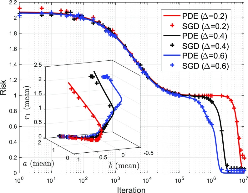
Multilayer neural networks are among the most powerful models in machine learning, yet the fundamental reasons for this success defy mathematical understanding. Learning a neural network requires optimizing a nonconvex high-dimensional objective (risk function), a problem that is usually attacked using stochastic gradient descent (SGD). Does SGD converge to a global optimum of the risk or only to a local optimum? In the former case, does this happen because local minima are absent or because SGD somehow avoids them? In the latter, why do local minima reached by SGD have good generalization properties? In this paper, we consider a simple case, namely two-layer neural networks, and prove that-in a suitable scaling limit-SGD dynamics is captured by a certain nonlinear partial differential equation (PDE) that we call distributional dynamics (DD). We then consider several specific examples and show how DD can be used to prove convergence of SGD to networks with nearly ideal generalization error. This description allows for "averaging out" some of the complexities of the landscape of neural networks and can be used to prove a general convergence result for noisy SGD.

Keywords: Wasserstein space; gradient flow; neural networks; partial differential equations; stochastic gradient descent.

Fig. 1.

Evolution of the radial distribution ${\overline{\rho }}_t$ for the isotropic Gaussian model, with $\mathrm{\Delta }=0.8$. Histograms are obtained from SGD experiments with $d=40$, $N=800$, initial weight distribution ${\rho }_0=\mathsf{\text{N}}\left(\mathbf{0},0.8^2/d\cdot {\mathbf{I}}_d\right)$, and step size $ϵ=10^{-6}$ and $\xi \left(t\right)=1$. Continuous lines correspond to a numerical solution of the DD (Eq. 13).

Fig. 2.

Population risk in the problem of separating two isotropic Gaussians, as a function of the separation parameter $\mathrm{\Delta }$. We use a two-layer network with piecewise linear activation, no offset, and output weights equal to 1. Empirical results obtained by SGD (a single run per data point) are marked “+.” Continuous lines are theoretical predictions obtained by numerically minimizing $R\left(\rho \right)$ (see SI Appendix for details). Dashed lines are theoretical predictions from the single-delta ansatz of Eq. 14. Notice that this ansatz is incorrect for $\mathrm{\Delta }>{\mathrm{\Delta }}_d^{\mathrm{h}}$, which is marked as a solid round dot. Here, $N=800$.

Fig. 3.

Evolution of the population risk for the variable selection problem using a two-layer neural network with ReLU activations. Here $d=320$, $s_0=60$, and $N=800$, and we used $\xi \left(t\right)=t^{-1/4}$ and $\epsilon =2\times 10^{-4}$ to set the step size. Numerical simulations using SGD (one run per data point) are marked +, and curves are solutions of the reduced PDE with $d=\infty$. (Inset) Evolution of three parameters of the reduced distribution ${\overline{\rho }}_t$ (average output weights $a$, average offsets $b$, and average ${\ell }_2$ norm in the relevant subspace $r_1$) for the same setting.

Fig. 4.

Separating two isotropic Gaussians, with a nonmonotone activation function (see Predicting Failure for details). Here $N=800$, $d=320$, and $\mathrm{\Delta }=0.5$. The main frame presents the evolution of the population risk along the SGD trajectory, starting from two different initializations of ${\left({\mathbf{w}}_i^0\right)}_{i\le N}{\sim }_{iid}\mathsf{N}\left(\mathbf{0},{\kappa }^2/d\cdot {\mathbf{I}}_d\right)$ for either $\kappa =0.1$ or $\kappa =0.4$. In Inset, we plot the evolution of the average of $\Vert \mathbf{w}{\Vert }_2$ for the same conditions. Symbols are empirical results. Continuous lines are predictions obtained with the reduced PDE (Eq. 13).

References

-
- Rosenblatt F. Principles of Neurodynamics. Spartan Book; Washington, DC: 1962.
- Krizhevsky A, Sutskever I, Hinton GE. Imagenet classification with deep convolutional neural networks. In: Vardi MY, editor. Advances in Neural Information Processing Systems. Association for Computing Machinery; New York: 2012. pp. 1097–1105.
- Goodfellow I, Bengio Y, Courville A, Bengio Y. Deep Learning. Vol 1 MIT Press; Cambridge: 2016.
- Robbins H, Monro S. A stochastic approximation method. Ann Math Stat. 1951;22:400–407.
- Bottou L. Large-scale machine learning with stochastic gradient descent. In: Lechevallier Y, Saporta G, editors. Proceedings of COMPSTAT’2010. Physica; Heidelberg: 2010. pp. 177–186.
Publication types
LinkOut - more resources
Full Text Sources
Other Literature Sources
Molecular Biology Databases
Miscellaneous