Global land change from 1982 to 2016

Abstract

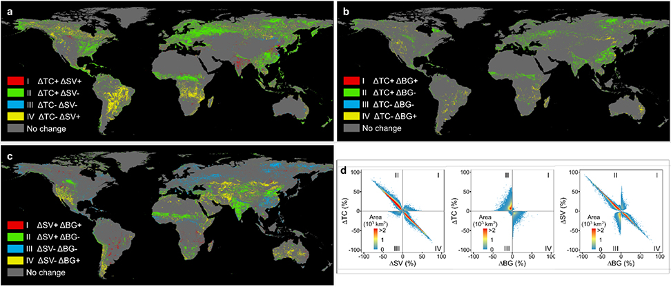
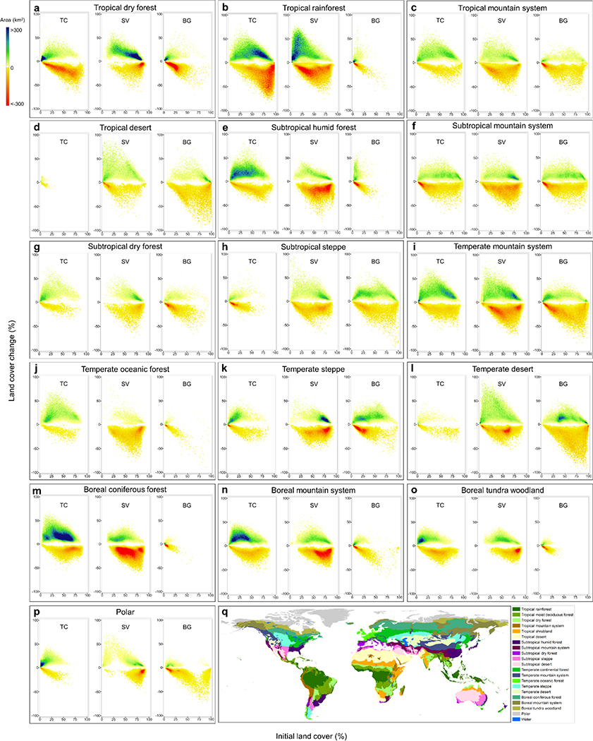
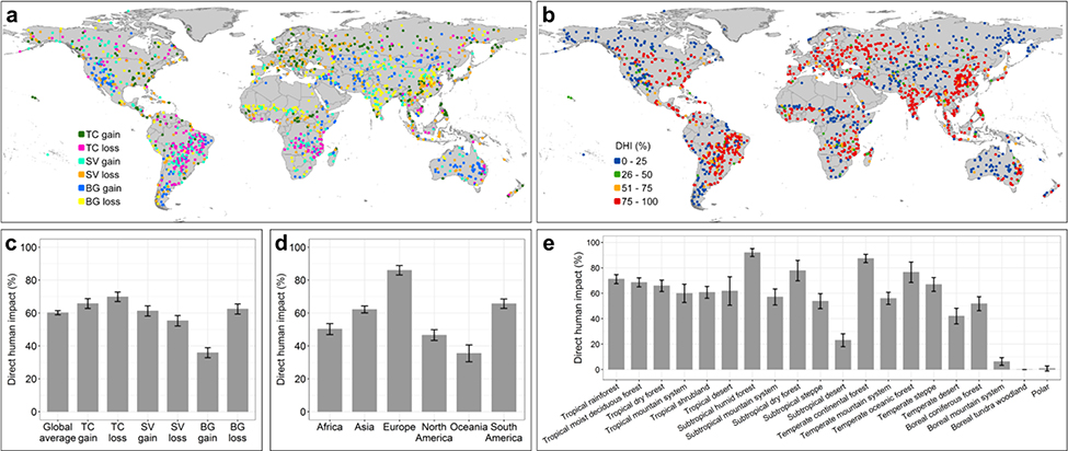
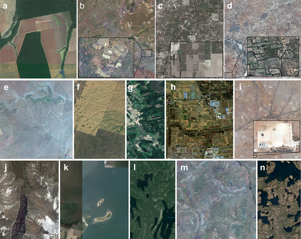
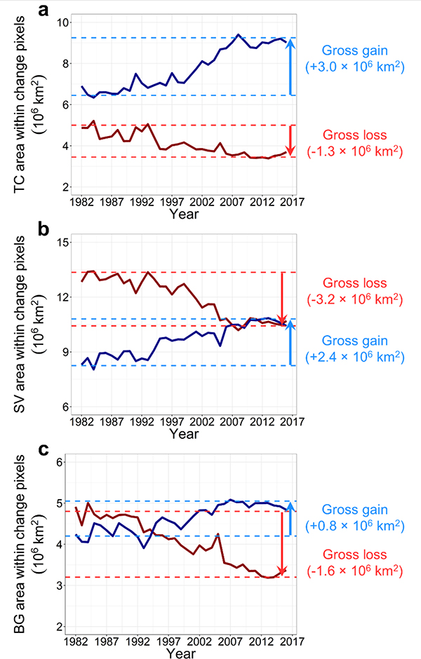
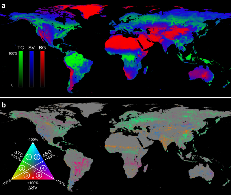
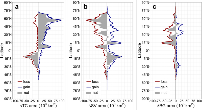
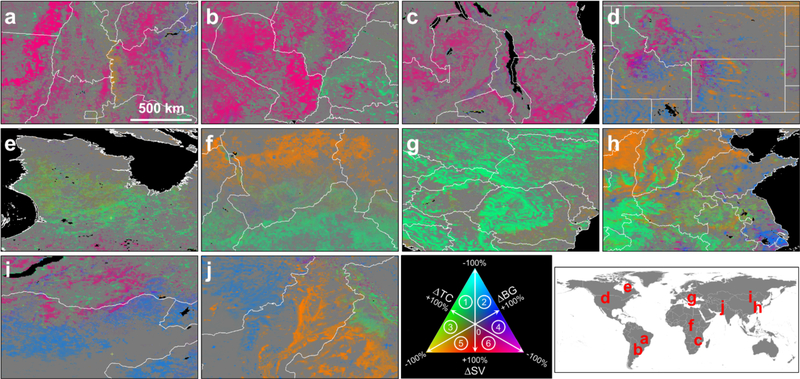
Land change is a cause and consequence of global environmental change^1,2. Changes in land use and land cover considerably alter the Earth's energy balance and biogeochemical cycles, which contributes to climate change and-in turn-affects land surface properties and the provision of ecosystem services^1-4. However, quantification of global land change is lacking. Here we analyse 35 years' worth of satellite data and provide a comprehensive record of global land-change dynamics during the period 1982-2016. We show that-contrary to the prevailing view that forest area has declined globally⁵-tree cover has increased by 2.24 million km² (+7.1% relative to the 1982 level). This overall net gain is the result of a net loss in the tropics being outweighed by a net gain in the extratropics. Global bare ground cover has decreased by 1.16 million km² (-3.1%), most notably in agricultural regions in Asia. Of all land changes, 60% are associated with direct human activities and 40% with indirect drivers such as climate change. Land-use change exhibits regional dominance, including tropical deforestation and agricultural expansion, temperate reforestation or afforestation, cropland intensification and urbanization. Consistently across all climate domains, montane systems have gained tree cover and many arid and semi-arid ecosystems have lost vegetation cover. The mapped land changes and the driver attributions reflect a human-dominated Earth system. The dataset we developed may be used to improve the modelling of land-use changes, biogeochemical cycles and vegetation-climate interactions to advance our understanding of global environmental change^1-4,6.

Extended Data Figure 1.

Satellite-derived, long-term (1982–2016) tree canopy cover change (ΔTC), short vegetation cover change (ΔSV) and bare ground cover change (ΔBG) show strong coupling and symmetry in change detection. a, Global map of co-located ΔTC and ΔSV. Pixels showing a statistically significant trend (Mann-Kendall test, p < 0.05) in both TC and SV are depicted on the map. b, Global map of co-located ΔTC and ΔBG. c, Global map of co-located ΔSV and ΔBG. d, From left to right, intensity plot of change area for ΔTC vs. ΔSV, ΔTC vs. ΔBG and ΔSV vs. ΔBG, corresponding to a, b and c respectively. To create these intensity plots, paired percent change layers (Fig. 1b) are used to construct a 2D histogram with bin size of 1% for both axes. Then, the total change area in each bin is calculated and plotted.

Extended Data Figure 2.

Long-term (1982–2016) gross change dynamics of tree canopy (TC) cover, short vegetation (SV) cover and bare ground (BG) cover vary considerably between biomes (a-p). Mountain systems (c, f, i, n) all exhibit larger area of TC gain than TC loss, larger area of SV loss than SV gain and larger area of BG loss than BG gain. q, Geographical distribution of all biomes. See Extended Data Table 2 for change area estimates.

Extended Data Figure 3.

Attributing direct human impact (DHI) versus indirect drivers to detected tree canopy (TC) cover change, short vegetation (SV) cover change, and bare ground (BG) cover change. Indirect drivers include both natural drivers and human-induced climate change. a, Spatial distribution of the probability sample used for the attribution estimates (n = 1500). b, DHI of each sample unit interpreted using a time-series of high resolution images in Google Earth. c, Estimated direct human impact at the global scale. Global average is calculated by weighting the human impact of each type by each respective global total area provided in Extended Data Table 1. Error bars represent the standard error (SE) for the estimated percent of direct human impact. d and e, Estimated direct human impact at the continental and biome scales.

Extended Data Figure 4.

Selected sample examples for driver attribution. Screenshots are taken from Google Earth. Each panel is 0.05° × 0.05° in size, corresponding to one AVHRR pixel. a, Deforestation for industrial agriculture expansion in Mato Grosso, Brazil (11.275°S, 52.125°W); b, Expanding shifting agriculture in northern Zambia (11.625°S, 28.625°E) c, Intensification of small-holder agriculture in Punjab, Pakistan (30.025°N, 71.675°E); d, Short vegetation gain in low-intensity agricultural lands in northern Nigeria (12.825°N, 7.825°E), e, Short vegetation increase due to effective fire suppression in pasture lands in Omaheke, Namibia (22.175°S, 18.925°E); f, Managed pasture lands in western Kazakhstan (49.475°N, 47.725°E), g, Forestry in southern Finland (61.075°N, 24.475°E), h, Urbanization in Shanghai, China (30.925°N, 121.175°E). i, Oil extraction in New Mexico, USA (32.875°N, 104.275°W). j, Herbaceous vegetation increase due to glacial retreat in Chuy, Kyrgyzstan (42.575°N, 74.775°E); k, Bare ground cover variation along Mar Chiquita lake shore in Cordoba, Argentina (30.675°S, 63.025°W). l, Forest fires in Saskatchewan, Canada (55.225°N, 102.225°W); m, Tree cover increase in unpopulated savannas in Western Equatoria, South Sudan^, (6.575°N, 27.725°E); n, Climate change-driven woody encroachment in Quebec, Canada (59.475°N, 73.225°W). Examples a-i show various types of land use, whereas examples j-n do not show visible signs of human activity.

Extended Data Figure 5.

Global trends in (a) tree canopy (TC) cover, (b) short vegetation (SV) cover, and (c) bare-ground (BG) cover during 1982–2016. The following steps were taken for each cover type using TC as the example. The TC gain layer (Fig. 1b) was overlaid on the annual TC% stack to compute annual global TC area within the gain mask (solid dark blue lines); the TC loss layer (Fig. 1b) was overlaid on the annual TC% stack to compute annual global TC area within the loss mask (solid dark red lines). Gross gain (loss) estimates between 1986 and 2016 are marked by blue (red) arrows and dashed lines. See Extended Data Table 1 for exact gross change estimates.

Extended Data Figure 6.

Adjusting systematic biases in annual AVHRR metrics using multi-year MODIS median as reference. The metric displayed in (a) is mean NDVI between 75 and 100 percentiles. This metric is related to the local peak growing season and was the most important variable driving the derived regression tree models for bare ground cover estimation. The metric displayed in (b) is mean red reflectance between 0 and 25 percentiles. This metric is also related to the local peak growing season and was the most important variable for tree cover estimation. For both (a) and (b), the dot plots on the left show the normalized and unnormalized, annual, global mean values, excluding Antarctica and Greenland, and the density scatter plots on the right show pixel-level comparison between years 1999 and 2001 before (upper figure) and after normalization (lower figure). Normalizing AVHRR using MODIS as reference not only changes the absolute value and data range of each individual year, but also enhances year-to-year consistency. c, Maps of the intact forest landscape (upper figure, green) and deserts (lower figure, orange) that are used as stable targets for normalization.

Extended Data Figure 7.

Accuracy assessment of AVHRR tree canopy (TC) cover, bare ground (BG) cover and short vegetation (SV) cover, based on a validation sample of 475 AVHRR pixels. a, Spatial distribution of the validation sample (red dot) overlaid on long-term (1982–2016) mean tree cover. The USGS tree cover reference data (5-km × 5-km, Universal Transverse Mercator projection) have greater spatial details (colored squares in b and c) due to their sub-meter resolution but have geolocation mismatch with the AVHRR product (0.05° × 0.05°, gray-scale squares in b and c) due to different projections. d, Temporal distribution of the USGS tree cover sample. e, Scatter plots of AVHRR tree cover against USGS reference tree cover. AVHRR and reference are matched by year and center coordinates. f-h, Scatter plots of AVHRR TC, BG and SV (year 2001) against Landsat-based estimates, which are free from geolocation mismatch. i, Quantitative error metrics, including conventional confusion matrices as well as root-meansquare-error (RMSE), mean absolute error (MAE), mean error (ME) and r². The standard error (SE) for the estimated error metrics is provided in the parentheses.

Extended Data Figure 8.

Uncertainty of tree cover change (ΔTC) and bare ground change (ΔBG). a, Spatial distribution of annual mean root-mean-square-deviation (RMSD) of TC between 1982 and 2016. b, Spatial distribution of annual mean RMSD of BG between 1982 and 2016. c, Spatial distribution of ΔTC uncertainty. d, Spatial distribution of ΔBG uncertainty. e, Normalized frequency distribution of ΔTC uncertainty. f, Normalized frequency distribution of ΔBG uncertainty. TC, BG and associated RMSD are outputs of regression tree models. Uncertainty is represented by the ratio of long-term TC (BG) change estimates to associated RMSD estimates. Positive values of the ratio metric represent uncertainty of gain and negative values represent uncertainty of loss. A greater absolute value indicates lower uncertainty and vice versa. Area under the frequency distribution equals 1. The frequency distributions suggest that tree cover gain exceeds tree cover loss and bare ground loss exceeds bare ground gain for any threshold level (e.g. dashed lines), hence the observed trends (net gain in tree cover and a net loss in bare ground cover over the study period) are valid.

Figure 1.

A satellite-based record of global tree canopy (TC) cover, short vegetation (SV) cover and bare ground (BG) cover between 1982 and 2016. a, Mean annual estimates. b, Long-term change estimates. Both mean and change estimates are expressed as percent of pixel area at 0.05° × 0.05° spatial resolution. Pixels showing a statistically significant trend (Mann-Kendall test, p < 0.05) in either TC, SV or BG are depicted on the change map. Circled numbers in the color legend denote dominant change directions: 1: ΔTC+ with ΔSV-; 2: ΔBG+ with ΔSV-; 3: ΔTC+ with ΔBG-; 4: ΔBG+ with ΔTC-; 5: ΔSV+ with ΔBG- and 6: ΔSV+ with ΔTC-.

Figure 2.

Latitudinal profiles of land cover change between 1982 and 2016. a, tree canopy cover change (ΔTC). b, short vegetation cover change (ΔSV). c, bare ground cover change (ΔBG). Area statistics were calculated for every 1° latitude.

Figure 3.

Intensity plots of gross loss and gain area in tree canopy (TC) cover, short vegetation (SV) cover and bare ground (BG) cover during 1982–2016. a, Global-scale plots (upper-left color bar). Initial land cover (x-axis) is defined as mean value of the first five years 1982–1986. To create these plots, for each cover class, percent change layer (Fig. 1b) and initial cover layer are used to construct a 2D histogram with bin size of 1% for both axes. Then, total change area in each bin is calculated and plotted. Data points located towards the lower-right corner of the TC plot are more likely to be deforestation (that is, points with large initial tree cover and large reduction in tree cover). The concentrated blue region of the SV plots reflects cropland intensification. The green belt on the BG plot suggests that vegetation loss occurred across the entire range of BG coverage. The dominance of TC gain over TC loss, SV loss over SV gain and BG loss over BG gain are also clearly revealed; b, Geographical distribution of four highlighted biomes with largest gross areal changes; c, largest gross TC loss and SV gain; d, largest gross TC gain and SV loss; e, largest gross BG loss; f, largest gross BG gain. The lower-left color bar is consistent across biomes (c-f) and cover types. Long-term gross dynamics of TC, SV and BG changes vary considerably between biomes. See Extended Data Fig. 2 for other biomes and Extended Data Table 2 for change area estimates.

Figure 4.

Regional subsets of changes in tree canopy (TC) cover, short vegetation (SV) cover and bare ground (BG) cover. a, Cerrado ecoregion in Brazil, centered at (11.4°S, 46.5°W). b, Gran Chaco ecoregion in Bolivia, Argentina and Paraguay, centered at (22.5°S, 55.7°W). c, Miombo woodlands in southeast Africa, centered at (12.4°S, 33.9°E). d, Western United States, centered at (44.5°N, 110.0°W). e, Quebec, Canada, centered at (57.9°N, 71.6°W). f, Central Africa, centered at (10.4°N, 19.4°E). g, Eastern Europe, centered at (46.1°N, 20.3°E). h, Eastern China, centered at (35.0°N, 115.1°E). i, Eastern Mongolia, centered at (48.7°N, 111.0°E). j, Afghanistan and Pakistan, centered at (30.7°N, 70.6°E). Circled numbers in the color legend denote dominant change directions: 1: ΔTC+ with ΔSV-; 2: ΔBG+ with ΔSV-; 3: ΔTC+ with ΔBG-; 4: ΔBG+ with ΔTC-; 5: ΔSV+ with ΔBG- and 6: ΔSV+ with ΔTC-.

References

1. Turner BL, Lambin EF & Reenberg A The emergence of land change science for global environmental change and sustainability. Proc. Natl. Acad. Sci. USA 104, 20666–20671 (2007). - PMC - PubMed
1. Foley JA et al. Global consequences of land use. Science 309, 570–574 (2005). - PubMed
1. Le Quéré C et al. Global carbon budget 2016. Earth Syst. Sci. Data 8, 605–649 (2016).
1. Alkama R & Cescatti A Biophysical climate impacts of recent changes in global forest cover. Science 351, 600–604 (2016). - PubMed
1. FAO. Global Forest Resources Assessment 2015. (UN Food and Agriculture Organization, Rome, Italy, 2015).
Publication types
MeSH terms
LinkOut - more resources