RNA velocity of single cells

Abstract

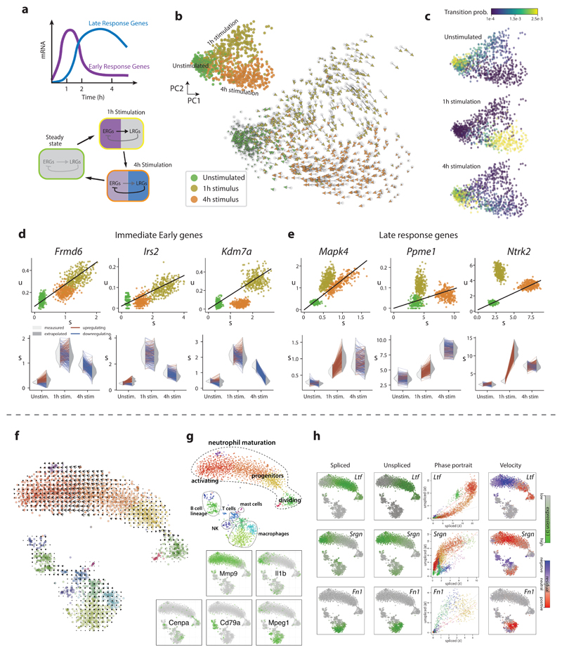
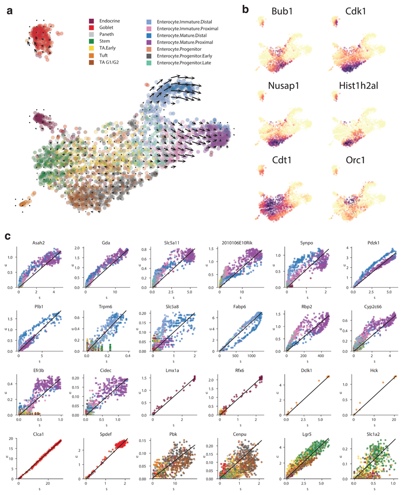
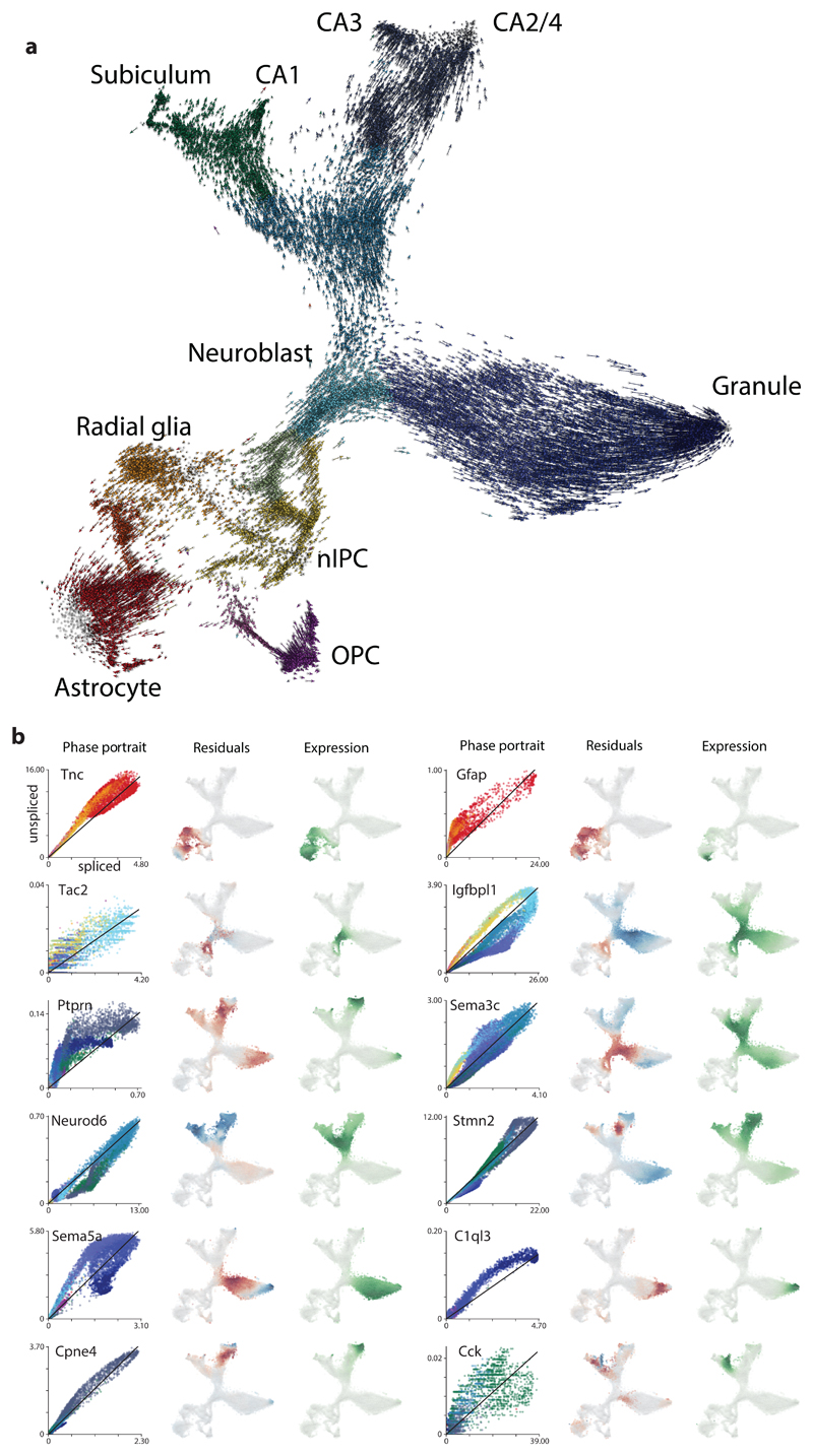
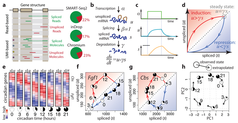
RNA abundance is a powerful indicator of the state of individual cells. Single-cell RNA sequencing can reveal RNA abundance with high quantitative accuracy, sensitivity and throughput¹. However, this approach captures only a static snapshot at a point in time, posing a challenge for the analysis of time-resolved phenomena such as embryogenesis or tissue regeneration. Here we show that RNA velocity-the time derivative of the gene expression state-can be directly estimated by distinguishing between unspliced and spliced mRNAs in common single-cell RNA sequencing protocols. RNA velocity is a high-dimensional vector that predicts the future state of individual cells on a timescale of hours. We validate its accuracy in the neural crest lineage, demonstrate its use on multiple published datasets and technical platforms, reveal the branching lineage tree of the developing mouse hippocampus, and examine the kinetics of transcription in human embryonic brain. We expect RNA velocity to greatly aid the analysis of developmental lineages and cellular dynamics, particularly in humans.

Extended Data Figure 1. Most of the intronic reads arise due to internal priming from stable positions.

a-d. Examples of read density around intronic polyA and polyT sequences. The browser screenshots show density of reads from the 10x Chromium mouse hippocampus dataset (top track of each panel), mouse bone marrow inDrop dataset (second track from the top), and chromaffin differentiation assessed using SMART-seq2 (third track). The bottom two tracks show gene annotation, and positions of polyA or polyT sequences (of length at least 15bp with one allowed mismatch). The polyA/polyT boxes are colored blue if the stretch is in a concordant orientation to the transcription of the underlying gene (i.e. would result in a polyA sequence in the nascent RNA molecule being transcribed), or red if they are oriented in the discordant position (i.e. would result in a polyT sequence in the RNA). The 3’-end based 10x Chromium and inDrop protocols show discrete peaks downstream of the polyA priming sites, with the 10x dataset also showing peaks upstream of the polyT sites. The SMART-seq2 protocol shows much more diffused peaks, expected from the full-length purification procedure used by the protocol. e-h. Average read density profiles around concordant and discordant internal priming sites. The plots show observed/expected intronic read density around (A)₁₅ or (T)₁₅ sequences (with 1 allowed mismatch) within the intronic regions. The x axis shows position relative to the motif position (in basepairs), in a genomic reference orientation. The bold lines show genome-wide average (trimmed of two extreme values among chromosomes for each position). The averages of individual chromosomes are shown semi-transparent lines. (e.) shows the profiles of mouse hippocampus 10x Chromium dataset (n=18,213), (f.) shows profile for human forebrain 10x data (n=1720), (g.) shows profile for the chromaffin differentiation data measured using SMART-seq2 (n=385), and (h.) shows profile for the mouse bone marrow data measured using inDrop (n=3018). The top left corner of each plot shows the number of all intronic reads (i.e. falling within the gene, but not touching an exon) that falls within the 250bp around internal priming sites (1500bp was used for the SMART-seq2 dataset). In 10x data, while concordant internal priming sites produce stronger signal, their frequency within the genome is lower than those of discordant sites, so that overall discordant sites account for slightly higher fraction of intronic signals. By contrast, the inDrop dataset appears to have very limited discordant priming.

Extended Data Figure 2. Estimation of the characteristic time of RNA metabolism in human cells.

a. Design of the metabolic labeling experiment in human cells. HEK 293 cells were exposed to 4sU for 5, 15 or 30 min, the labeled fraction was isolated and analyzed. A no pull-down control was also analyzed, and represents the equilibrium state (indicated by ∞). b. Expected profiles of the abundance and fraction of labeled spliced and unspliced RNA molecules. c. The observed dynamic profiles of genes were clustered, yielding two groups: the majority (83.4%) were concordant with the expectation of increasing labeling; and a smaller fraction (16.6%) of discordant genes. Bars indicate SEM. n_genes=998, N_technical=2 N_biological=2. d. Curves showing maximum likelihood fit to the data, based on the analytical solution for a step increase of the transcription rate. The fit yields values of β and γ, and of the characteristic time constant τ, defined as the time required to reach 1 – 1 /e ≈ 63.2 % of the asymptotic value. e. The distribution of τ values and f. The joint distribution of the fit β and γ parameters (n=832).

Extended Data Figure 3. Degradation rates are conserved over a wide range of terminally differentiated cell types.

Conservation of the RNA degradation rate over a wide range of different cell types in the adult mouse (Tabula Muris dataset). a. The distribution over the genes of the correlation of spliced and unspliced molecule counts across all the cell types (n_genes=8,385). b. Legend enumerating the tissues and cell classes annotated by the Tabula Muris consortium (n=48). Functionally, developmentally or phenotypically related are colored with similar colors to aid the interpretation of the plots below. c. A representative selection of genes with high correlation (ρ > 0.9) and d. typical correlation (0.9 > ρ > 0.4). γ was estimated by robust linear regression (RANSAC) e. Plots show a selection of genes displaying two clearly distinct degradation rates (such genes with double γ amounted to 10.8% of the total). The values of the two different γ were estimated by regression mixture modeling. f,g. Two examples of genes where multiple gammas are explained by alternative splicing in different cell types.

Extended Data Figure 4. Structure-based velocity estimation.

a,b. For genes that are observed only outside of the steady state, such as genes upregulated late in the chromaffin differentiation (a) or down-regulated early in the Schwann cell precursors (b), gene-relative γ fit will likely deviate from its steady-state value. c,d. To correct for such effects, a structure-based γ fit will first predict γ for every gene based on its structural parameters, and then use k most correlated genes in the dataset to adjust M-value (M = log₂[u_o/u_ss], where u_ss is the unspliced counts predicted from spliced counts under steady-state, and u_o is the observed unspliced count) using robust mean, and re-estimate γ. e. Scatter-plot comparing gene-relative and structure-based γ estimates, with colored circles highlighting γ adjustments for genes down-regulated early in SCPs (blue) and up-regulated late in chromaffin cells (green). The values are shown on a natural log scale. f-i. Cell expression velocity in the chromaffin E12.5 dataset, based on the structure-based γ estimates, shown on the first five PCs.

Extended Data Figure 5. RNA velocity analysis of inDrop datasets: visual stimulus response of cortical pyramidal neurons and neutrophil differentiation.

a. Simplified illustration of a model of activation of pyramidal neurons of the visual cortex after exposure to a light stimulus. b. Velocity estimates projected onto a two-dimensional PCA embedding of the dataset (n=952) c. Average transition probability of unstimulated cells (top), cells stimulated for 1h (middle) and cell stimulated for 4h (bottom). The unstimulated cells mostly were stationary and only few cells show tendency of activating early response genes (likely as a result of the dissociation procedure). Cells stimulated for 1h were characterized by expressing immediate early genes and high velocity in late response genes, and they were therefore transitioning to a state more similar to the one observed 4h activation time point. After 4h of stimulations cells appeared to be reverting to a state comparable to the unstimulated sample (bottom). d,e. Above, phase portraits of early (d) and late (e) response genes. Below, Violin plots show expression distribution over the cell population at each time point (left half of the violin) and extrapolation in to the future using velocity (right half of the violin). In the plot, transitions of single cells are indicated by lines connecting the two halves of the violins and colored by the sign of the velocity of each gene. f. Grid visualization shows cell expression velocity estimates for the inDrop mouse bone marrow dataset on a t-SNE embedding (n=3018). g. Major cell populations are labeled based on manual annotation. The velocity flow in (a) captures neutrophil maturation, starting from the dividing cells on the right, all the way to Il1b activation on the left. Expression profiles for five marker genes are shown below. h. The plots illustrate gene-relative model fits for several example genes. For each gene, the first column shows spliced molecular counts in different cells. The second column shows unspliced molecular counts. Third column shows phase portrait of a gene (unspliced vs. spliced dependency) and the resulting γ fit (dashed red line), as determined using extreme quantile method. Each point corresponds to a cell, colored according to cluster labels shown in (g). The last column shows unspliced count signal residual based on the estimated γ fit, with positive residuals indicating expected upregulation, and negative residuals indicating expected downregulation of a gene.

Extended Data Figure 6. Dynamics of maturation of enterocytes during intestinal homeostasis.

a. Velocity field projected on a 2D t-SNE embedding. The clusters are labeled and colored as in the original publication to facilitate comparison (n=2683). Velocity analysis revealed a transition related to the maturation of distal and proximal enterocytes. No consistent velocity was observed in the part of the manifold occupied by stem cells and transit amplifying (TA) cells, suggesting that stem cell dynamics is more difficult to capture either for its slower rate or a more stochastic nature. The small velocities of transit amplifying cells were likely driven by cell cycle process. b. A selection of the cell cycle genes that were removed in the analysis are plotted on the t-SNE. Despite the removal of the genes annotated as cell cycle genes we still observed important segregation by cell cycle, illustrating the difficulty of disentangling cell cycle phase from the cell state. c. A selection of phase portraits that show genes underlying the observed velocity field. Markers of Endocrine, Goblet and Tuft cells displayed no detectable velocity. Velocity towards and from stem cell states was detectable for limited set of genes (like the stem cell marker Lgr5), however on the genome-wide level the exact dynamics of this process was likely confounded by the high correlation with cell cycle.

Extended Data Figure 7. RNA velocity unveils the dynamics of differentiation and myelination of oligodendrocytes.

a. t-SNE projection shows the landscape of oligodendrocyte lineage differentiation and myelination process in the hindbrain (pons) of adolescent (P20) mice (n=6307). The velocity field reflects the dynamics of expression of both the initial differentiation wave and the following expression changes associated to the myelination process. The cell clusters are colored by pseudotime as in (c) to facilitate interpretation. b. Expression patterns of landmark genes of the differentiation process. Pdgfra is the canonical marker of oligodendrocyte precursors (OPCs), Neu4 marks committed oligodendrocyte precursors (COPs), Tmem2 is enriched in newly formed oligodendrocyte (NFOLs) and the expression of Mog is upregulated at the beginning of the myelination process in myelin forming oligodendrocytes (MFOLs). c. A selection of phase portraits underlying the velocity field showed in (a). d. t-SNE projections and velocity vector field of the same dataset, but analyzed using a more naïve feature selection that has retained other axes of variation on top of the oligodendrocyte maturation (sex and day of dissection). Notice that despite separation of populations into Xist+ and Xist- tracks, the velocity field correctly captures progression from progenitors to newly formed oligodendrocytes in the two parallel tracks. e. Level of expression of Xist showing that most of the extra variation is driven by the sex of the animal. f. Cells colored by the day the experiment was performed in.

Extended Data Figure 8. Agreement of velocity predictions with the observed expression derivatives.

a. Maturation progression of granule neurons in the mouse hippocampus dataset is approximated by pseudotime (estimated with a principal curve). b. For a pair of example genes (rows), the plots show unspliced and spliced gene expression profiles along the pseudotime (left panels), empirically-estimated smoothed pseudotime derivative of the observed gene expression and the estimated RNA velocity (middle panels), as well as the relationship between spliced and unspliced expression (right panel). The velocity estimates for the two chosen genes are highly correlated with the empirically-observed derivative, indicating accurate velocity estimation. c. The majority (75%) of the genes that were differentially regulated along the pseudotime trajectory showed positive correlation with the empirical expression derivative. The distribution of such genes is split according to three classes of trajectory-associated genes as shown in d. By contrast, velocity estimates for genes that were not differentially expressed along the pseudotime trajectory did not show such correlation (grey). Incorporating information about co-regulated genes into velocity estimation using gene kNN clustering (see Supplementary Note 1) can significantly boost the accuracy of the velocity predictions (lower panel). d. Trajectory-associated genes were classified as early, transient and late, according to their peak expression time. x-axis: cells ordered by pseudotime, y-axis: genes ordered by their peak expression time. e. The genes that were well-correlated in terms of their spliced expression patterns with Ptprg, also showed high correlation of their velocity estimates with Ptprg. To assess the degree consistency of the velocities of co-regulated genes, we introduced a measure of velocity coordination for a given gene, as a difference between the mean correlations of the velocity estimates of the co-regulated genes and the velocity estimates of all genes. The two quantities being compared are shown for Ptprg with dotted vertical lines: grey – mean velocity correlation with all genes, red – mean velocity correlation with top co-regulated genes. Velocity coordination provides an unbiased measure of quality of velocity estimates. f. Velocities of co-regulated genes were correlated. Distribution of gene velocity coordination values is shown for genes that had co-regulated genes (i.e. the genes that had well-correlated gene neighbors in terms of their spliced expression pattern, green), as well as for the genes that did not have enough co-regulated genes (without neighbors, grey). g. Co-regulated genes that had high velocity coordination tended to have high correlation with the empirical derivatives. Spearman correlation coefficient is shown. h-k. Velocity performance during maturation of pyramidal neurons (h). Genes differentially expressed during maturation had high correlation of velocity with empirical derivative (i), co-regulated genes tended to have correlated velocity estimates (j) and the degree of velocity coordination was associated with its correlation with empirical derivative (k). l-m. Velocity performance during chromaffin differentiation. p-s. Velocity performance during maturation of oligodendrocytes. Number of top co-regulated genes analyzed for velocity correlation: (g): 200 genes, (k,o,s): 150 genes.

Extended Data Figure 9. Branching developmental trajectories of developing hippocampus.

a. t-SNE embedding of the developmental dentate gyrus dataset. Cells are colored by cluster identities, with labels shown for the major cell types. b. Expression of radial glia (and astrocyte) marker Hes1, and cell cycle genes Top2a and Cdk1 shown on the t-SNE embedding. c. Marker genes of different regions of the hippocampus (in situ hybridization images from Allen Brain Atlas) show prominent expression signals at different extremities of the branching embedding. Scale bars, 0.5 mm.

Extended Data Figure 10. Single cell velocity estimates for individual cells in the embryonic hippocampus dataset.

a. Arrows indicate the extrapolated state projected onto the t-SNE embedding of the manifold. b. Selected phase portraits and fits of the equilibrium slope (γ) for the developing cells in the embryonic hippocampus dataset. For each gene, the first column shows spliced-unspliced phase portrait. The dashed line shows the γ fit. The second column illustrates the magnitude of the residuals (i.e. difference between observed and expected unspliced abundance, which closely tracks with velocity) for several genes involved in the development of different neural lineages. The third column shows the observed expression profile for spliced molecules.

Figure 1. Balance between unspliced and spliced mRNAs is predictive of cellular state progression.

a. Spliced and unspliced counts are estimated by separately counting reads that incorporate intronic sequence. Multiple reads associated with a given molecule are grouped (* boxes) for UMI-based protocols. Pie charts show typical fractions of unspliced molecules. b. Model of transcriptional dynamics, capturing transcription (α), splicing (β), and degradation (γ) rates involved in production of unspliced (u) and spliced (s) mRNA products. c. Solution of the model in (b) as a function of time, showing unspliced and spliced mRNA dynamics in response to step changes in α. d. Phase portrait showing the same solution (solid curves). Steady states for different values of transcription rates α fall on the diagonal given by slope γ (dashed line). Levels of unspliced mRNA above or below that proportion indicate increasing (red shading) or decreasing (blue shading) expression of a gene, respectively. e. Abundance of spliced (s) and unspliced (u) mRNAs for circadian-associated genes in a 24h time course of mouse liver. The unspliced mRNAs are predictive of spliced mRNA at the next time point. f,g. Phase portraits observed for a pair of circadian-driven genes: Fgf1 (f) and Cbs (g). The circadian time of each point is shown using a clock symbol (see bottom of Fig. 1e). The dashed diagonal line shows steady-state relationship, as predicted by γ fit. h. Change in expression state at a future time t, as predicted by the model, is shown in the space of the first two principal components (PCs), recapitulating the progression along the circadian cycle. Each circle shows the observed expression state, with the arrow pointing at the position of the future state, extrapolated from velocity estimates.

Figure 2. RNA velocity recapitulates dynamics of chromaffin cell differentiation.

a. PCA projection showing major subpopulations of Schwann cell precursors (SCPs) differentiating into chromaffin cells in E12.5 mouse (n=385 cells). b,c. Expression pattern (left), unspliced/spliced phase portraits (center, cells colored according to a), and u residuals (right) are shown for the repressed Serpine2 (b) and induced Chga (c) genes. Read counts were pooled across k = 5 nearest cell neighbors. d. The observed and the extrapolated future (arrows) states are shown on the first two PCs. RNA velocity was estimated without cell or gene pooling. e. SCP-to-chromaffin cell transition as evidenced by lineage tracing with SCP-specific PLP1-CreERT2 line. A cross-section through the developing adrenal medulla is shown. Note high proportion of TH+/YFP+ cells in the developing medulla and the absence of such double-positive cells in the sympathetic ganglion (N=3 replicates). f. Extrapolation distance along the chromaffin differentiation trajectory is estimated for a single cell at pseudotime t₀, based on the correlation (y axis) between the velocity v and cell expression difference. Red line shows optimal extrapolation time (t*) (see Supplementary Note 2 Section 6). g. Distribution of optimal extrapolation times (t*- t₀) for the chromaffin differentiation timecrouse. Red line marks the distribution mode (2.1 hours). h. The velocities are visualized on the pre-defined t-SNE embedding from the original publication. Velocity estimates based on nearest-cell pooling (k = 5) were used. i. Same velocity field as (h) visualized using Gaussian smoothing on a regular grid.

Figure 3. RNA velocity field describes fate decisions of major neural lineages in the hippocampus.

a. A t-SNE embedding of the developing mouse hippocampus cells (n=18,213 cells), showing major transient and mature subpopulations. b. Phase portraits (left, colored as in a), unspliced residuals (middle), and spliced expression (right) are shown for two regulated genes. kNN cell pooling was used. c. Velocity field projected onto the t-SNE embedding. Arrows show the local average velocity evaluated on a regular grid. Upper right insert: differentiation endpoints as high density regions on the manifold after forward Markov process with velocity-based transition probabilities; the root of the branching tree is identified simulating the process in the reverse direction. Lower right insert: Summary schematic of the RNA velocity field, and expression of the transcription factor Prox1. d. Commitment to oligodendrocyte fate. Left, visualization of single-step transition probabilities from two starting cells (red) to neighbouring cells. Right, velocities of a sampled subset of cells shown on the t-SNE embedding in (c). e. Fate decision of neuroblasts. Left, visualization of single-step transition probabilities from two starting cells (red) to neighbouring cells. Right, velocities of a sampled subset of cells shown on the t-SNE embedding in (c).

Figure 4. Kinetics of transcription during human embryonic glutamatergic neurogenesis.

a. PCA projection of human glutamatergic neuron differentiation (n=1,720 cells) at post-conception week 10, shown with velocity field. Colors indicate cell types and intermediate states. A corresponding principal curve is shown in bold. b. Gene expression for known markers of radial glia (SOX2), neuroblasts (EOMES) and neurons (SLC17A7) and for novel markers are visualized on the PCA projection as in indicated genes in pseudocolor. c. Fluorescent in situ hybridization (RNAscope) for the same genes as in (b) on a cross-section of human developing cortex, oriented with the ventricular zone towards the bottom and the cortical surface towards the top (N=1). Scale bars, 25 μm. d. Pseudotime expression profiles for six example genes regulated in glutamatergic neuron maturation. Unspliced abundance was divided by γ to match the scale of spliced abundance.

References

1. Linnarsson S, Teichmann SA. Single-cell genomics: coming of age. Genome Biol. 2016;17:97. - PMC - PubMed
1. Zeisel A, et al. Coupled pre-mRNA and mRNA dynamics unveil operational strategies underlying transcriptional responses to stimuli. Mol Syst Biol. 2011;7:529. - PMC - PubMed
1. Gray JM, et al. SnapShot-Seq: A method for extracting genome-wide, in Vivo mRNA dynamics from a single total RNA sample. PLoS One. 2014;9 - PMC - PubMed
1. Gaidatzis D, Burger L, Florescu M, Stadler MB. Analysis of intronic and exonic reads in RNA-seq data characterizes transcriptional and post-transcriptional regulation. Nat Biotechnol. 2015;33:722–729. - PubMed
1. Picelli S, et al. Smart-seq2 for sensitive full-length transcriptome profiling in single cells. Nat Methods. 2013;10:1096–8. - PubMed
Publication types