The environmental niche of the global high seas pelagic longline fleet

Abstract

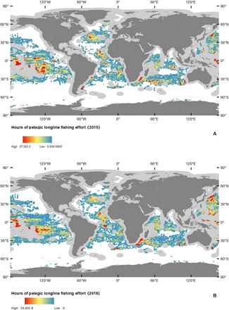
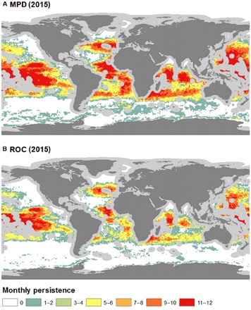
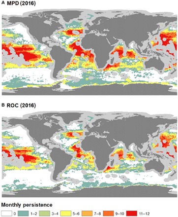
International interest in the protection and sustainable use of high seas biodiversity has grown in recent years. There is an opportunity for new technologies to enable improvements in management of these areas beyond national jurisdiction. We explore the spatial ecology and drivers of the global distribution of the high seas longline fishing fleet by creating predictive models of the distribution of fishing effort from newly available automatic identification system (AIS) data. Our results show how longline fishing effort can be predicted using environmental variables, many related to the expected distribution of the species targeted by longliners. We also find that the longline fleet has seasonal environmental preferences (for example, increased importance of cooler surface waters during boreal summer) and may only be using 38 to 64% of the available environmentally suitable fishing habitat. Possible explanations include misclassification of fishing effort, incomplete AIS coverage, or how potential range contractions of pelagic species may have reduced the abundance of fishing habitats in the open ocean.

Fig. 1. Distribution of global pelagic drifting longline fishing in ABNJ in 2015 and 2016.

(A) 2015. (B) 2016. Light gray areas depict exclusive economic zones (EEZs) that were excluded from this study. Fishing effort (hours) as calculated by GFW using satellite-based AIS data. Given the differences in quantified fishing effort between 2015 and 2016, the scales were maintained separate to showcase how, despite changes in intensity, the main trends in longline fishing effort are maintained. Gray areas around coastlines depict EEZs excluded from this study. Data are from GFW.

Fig. 2. Monthly distribution of pelagic longline fishing effort in ABNJ by the top five fishing States or territories, and all other countries combined.

The total calculated fishing effort between the years increases between 2015 and 2016, with China and Taiwan experiencing the largest increases in quantified fishing effort. ”*Other” represents a total of 45 other fishing nations deployed longline (LL) gear in ABNJ between 2015 and 2016.

Fig. 3. The monthly persistence of suitable habitat in ABNJ for 2015.

These persistence estimates were calculated using two different probability distribution cutoff thresholds: (A) MPD and (B) ROC. Gray areas around coastlines depict EEZs excluded from this study. Data are from GFW.

Fig. 4. The monthly persistence of suitable habitat in ABNJ for 2016.

These persistence estimates were calculated using two different probability distribution cutoff thresholds: (A) MPD and (B) ROC. Gray areas around coastlines depict EEZs excluded from this study. Data are from GFW.

Fig. 5. The average coefficient of variation of predicted high seas fishing suitability for 2015 and 2016.

Tropical latitudes show, on average, more predictive stability throughout the study period, whereas temperate and subpolar waters show higher degrees of variability of suitable habitat. Gray areas around coastlines depict EEZs excluded from this study. Data are from GFW.

Fig. 6. Radar plots of the average quarterly VI scores in 2015 and 2016.

(A) 2015. (B) 2016. The monthly VI scores for each of the two years assessed were averaged by quarter (Q) to capture the seasonal changes in the importance of each of the environmental predictors: Q1, January–March; Q2, April–June; Q3, July–September; Q4, October–December.

References

1. Swartz W., Sala E., Tracey S., Watson R., Pauly D., The spatial expansion and ecological footprint of fisheries (1950 to present). PLOS ONE 5, e15143 (2010). - PMC - PubMed
1. Sea Around Us Concepts, Design and Data, D. Pauly, D. Zeller, Eds. (2015); www.seaaroundus.org.
1. Sala E., Mayorga J., Costello C., Kroodsma D., Palomares M. L. D., Pauly D., Sumaila U. R., Zeller D., The economics of fishing the high seas. Sci. Adv. 4, eaat2504 (2018). - PMC - PubMed
1. United Nations Food and Agriculture Organization (FAO), The State of World Fisheries and Aquaculture 2014 (FAO, 2014).
1. Juan-Jordá M. J., Mosqueira I., Cooper A. B., Freire J., Dulvy N. K., Global population trajectories of tunas and their relatives. Proc. Natl. Acad. Sci. U.S.A. 108, 20650–20655 (2011). - PMC - PubMed
Publication types
LinkOut - more resources