Functional gradients of the cerebellum

Abstract

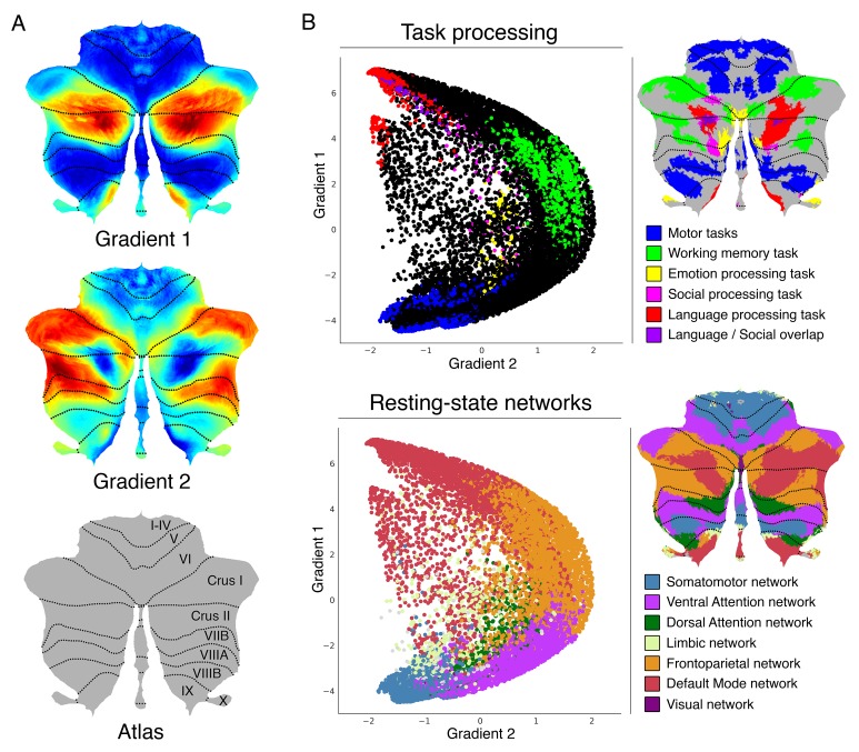
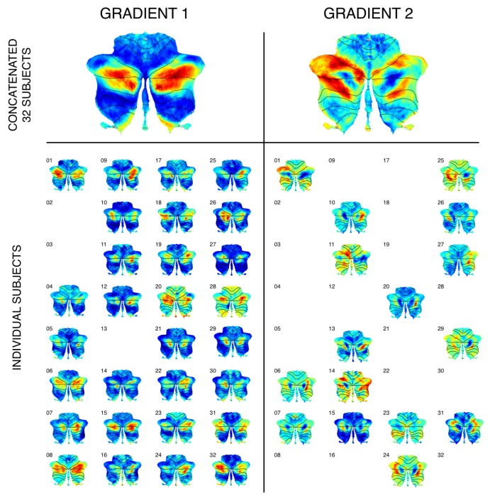
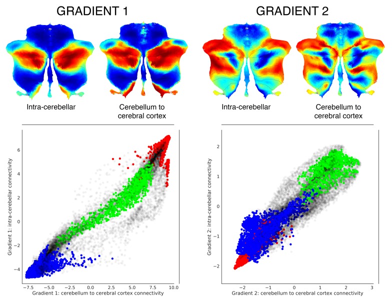
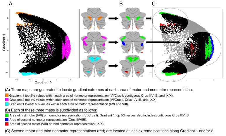
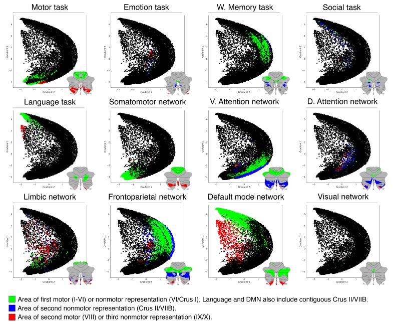
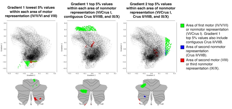
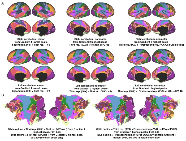
A central principle for understanding the cerebral cortex is that macroscale anatomy reflects a functional hierarchy from primary to transmodal processing. In contrast, the central axis of motor and nonmotor macroscale organization in the cerebellum remains unknown. Here we applied diffusion map embedding to resting-state data from the Human Connectome Project dataset (n = 1003), and show for the first time that cerebellar functional regions follow a gradual organization which progresses from primary (motor) to transmodal (DMN, task-unfocused) regions. A secondary axis extends from task-unfocused to task-focused processing. Further, these two principal gradients revealed novel functional properties of the well-established cerebellar double motor representation (lobules I-VI and VIII), and its relationship with the recently described triple nonmotor representation (lobules VI/Crus I, Crus II/VIIB, IX/X). Functional differences exist not only between the two motor but also between the three nonmotor representations, and second motor representation might share functional similarities with third nonmotor representation.

Keywords: cerebellum; fMRI; functional organization; functional topography; gradients; human; neuroscience; resting-state.

Figure 1.. Cerebellum gradients and relationship with discrete task activity maps (from Guell et al., 2018a) and resting-state maps (from Buckner et al., 2011).

Gradient 1 extended from language task/DMN to motor regions. Gradient 2 isolated working memory/frontoparietal network areas. (A) Cerebellum flatmap atlas and gradients 1 and 2. (B) A scatterplot of the first two gradients. Each dot corresponds to a cerebellar voxel, position of each dot along x and y axis corresponds to position along Gradient 1 and Gradient 2 for that cerebellar voxel, and color of the dot corresponds to task activity (top) or resting-state network (bottom) associated with that particular voxel.

Figure 1—figure supplement 1.. Schematic representation of diffusion map embedding.

(A) This example presents a schematic representation of diffusion map embedding. It illustrates the calculation of the principal functional gradient of 4 cerebellar voxels (red, green, blue, magenta) based on their functional connectivity with two target cerebellar voxels (yellow, orange). (B) Connectivity from each cerebellar voxel (red, green, blue, magenta) to the two target cerebellar voxels (yellow, orange) is represented as a two-dimensional vector. (C) All vectors can be represented in the same two-dimensional space. (D) Cosine distance between each pair of vectors is calculated, and (E) an affinity matrix is constructed as (1-cosine distance) for each pair of vectors. This affinity matrix represents the similarity of the connectivity patterns of each pair of voxels. (F) A Markov chain is constructed using information from the affinity matrix. Information from the affinity matrix is thus used to represent the probability of transition between each pair of vectors. In this way, there will be higher transition probability between pairs of voxels with similar connectivity patterns. This probability of transition between each pair of vectors can be analyzed as a symmetric transformation matrix, thus allowing the calculation of eigenvectors. (G) Eigenvectors derived from this transformation matrix represent the principal orthogonal directions of transition between all pairs of voxels. Here we illustrate the first resulting component of this analysis – the principal functional gradient of our four cerebellar voxels (red, green, blue, magenta) based on their connectivity with our two target cerebellar voxels (yellow, orange) progresses from the blue, to the green, to the magenta, to the red voxel. (H) This order is mapped back into our cerebellum map, allowing us to generate functional neuroanatomical descriptions. Of note, our cerebellar functional gradients were calculated using functional connectivity values of each cerebellar voxel with the rest of cerebellar voxels (rather than between four voxels and only two target cerebellar voxels, as in this example). Vectors in our analysis thus possessed many more than just two dimensions, but cosine distance can also be calculated between pairs of high-dimensional vectors. Diffusion map embedding using functional connectivity values from each cerebellar voxel to all cerebellar voxels thus captures the principal gradients of cerebellar functional neuroanatomy.

Figure 1—figure supplement 2.. Additional gradients.

Left: variance explained by each gradient; red diamonds correspond to the first eight gradients. Right: Gradients 1–8. Gradients 3 and 4 revealed laterality asymmetries in areas of nonmotor processing (Crus I, Crus II, VIIB and IX) but not in areas of motor processing (IV/V/VI and VIII). Notably, these asymmetries were constrained to areas of nonmotor processing (asymmetries are not present in motor lobules IV/V/VI and VIII). Consistent with this observation, left/right asymmetries in cerebellar processing have been described in multiple nonmotor tasks (Hu et al., 2008) but not in motor processing. One extreme of Gradient 5, 7 and 8 included unilateral or bilateral aspects of lobule IX (extreme shown in red for Gradient 5 and 8 and in blue for Gradient 7). Gradient 6 included at one extreme anterior portions of Crus I and Crus II. The other end included medial Crus I and Crus II as well medial regions of lobule VIIB. The added percentage of variability explained by each following gradient was minimal.

Figure 1—figure supplement 3.. Cerebellum gradients and relationship with discrete task activity for an individual subject (one resting-state run of 15 min).

(A) Top: Variance explained by each gradient; red diamonds correspond to the first four gradients. Bottom: Gradients 1–4 with 4 and 10 sigma (σ) values for smoothing of connectivity gradients. (B) A scatterplot of the first two gradients. Each dot corresponds to a cerebellar voxel, position of each dot along x and y axis corresponds to position along Gradient 1 and Gradient 2 for that cerebellar voxel, and color of the dot corresponds to task activity associated with that particular voxel. Scatterplots are shown for sigma = 4 (top) and sigma = 10 (bottom) values for smoothing of connectivity gradients. Task activity z maps are thresholded at z > 4 and include 4 mm spatial smoothing as provided by HCP, in addition to sigma = 2 smoothing using workbench command -cifti-smoothing.

Figure 1—figure supplement 4.. Cerebellum single-subject and group-level functional gradients calculations in a group of 32 participants.

Top row: Gradients 1 and 2 could also be observed when analyzing concatenated dataseries from a group of 32 participants, highlighting the applicability of our methodology to group studies with small cohorts of unrelated subjects. Bottom row: When calculating gradients within each individual participant of this subgroup and evaluating any of the first four resulting gradients, gradients with a distribution similar to gradient 1 could be observed in most cases (29 out of 32 participants). Gradients with a distribution similar to gradient 2 could be observed in half of the participants. Gradients are shown here only in cases where one of the first four components matched the distribution of gradient 1 or 2 for each subject. It is possible that additional components other than the first four contained a distribution similar to gradient 2. Future studies aiming to perform group comparison statistics using functional gradients would benefit from alternate alignment strategies (e.g. using Procrustes analysis; exploring this methodology is outside the scope of this article). Future studies may also analyze whether cerebellar functional gradients inter-subject variability can predict relevant behavioral aspects such as task performance, disease diagnosis, prognosis, or treatment response. Exploring such applications is also outside the scope of this article.

Figure 1—figure supplement 5.. Clustering of connectivity gradients revealed discrete networks similar to cerebello-cerebral connectivity parcellations from Buckner et al. (2011).

(A) Silhouette coefficient analysis revealed an optimal number of 14 and 18 clusters for k-means and spectral cluster, respectively. Both clustering approaches revealed a distribution of parcels similar to the 17-network cerebello-cerebral connectivity parcellation from Buckner et al. (2011). (B) K-means and spectral clustering using five clusters and gradients 1 and 2 revealed a distribution of parcels similar to the 7-network cerebello-cerebral connectivity parcellation from Buckner et al. (2011), as well as a pattern of inverted representations (inverted pattern indicated with an asterisk). We used five clusters instead of 7 given the relatively small representation of two of the networks (visual and limbic) in Buckner et al. (2011), and the first two gradients given that those reflect the double/triple representation distribution which is observed in the 7-networks map from Buckner et al. (2011). Note that while Buckner et al. (2011) applied a winner-takes-all algorithm to determine the strongest functional correlation of each cerebellar voxel to one of the 7 or 17 cerebral cortical resting-state networks, our analysis included cerebellum-to-cerebellum correlations only.

Figure 1—figure supplement 6.. Cerebral cortical resting-state networks from Yeo and colleagues (Yeo et al., 2011) (dark purple, visual; blue, somatomotor; green, dorsal attention; violet, ventral attention; cream, limbic; orange, frontoparietal; red, default network) revealed an overlap between DMN (red) and language task activity (grey) also in the cerebral cortex.

Language task activity map corresponds to Cohen’s d map thresholded at 0.5 from Guell et al. (2018a).

Figure 2.. Functional gradients calculated based on functional connectivity between the cerebellum and the cerebral cortex revealed a similar distribution when compared to intra-cerebellar functional gradients.

Left scatterplot represents intra-cerebellar gradient 1 (y axis) vs. cerebellum-to-cerebral-cortex gradient 1 (x axis). Right scatterplot represents intra-cerebellar gradient 2 (y axis) vs. cerebellum-to-cerebral-cortex gradient 2 (x axis). Scatterplot colors correspond to cerebellar task activation maps as shown in Figure 1: motor (blue), working memory (task-focused cognitive processing) (green), and language (task-unfocused cognitive processing) (red). As in the case of intra-cerebellar functional gradient 1 (left y axis), cerebello-cortical gradient 1 (left x axis) distinguishes motor (blue) vs. task-positive cognitive processing (green) vs. task-negative cognitive processing (red). Similarly, as in the case of intra-cerebellar functional gradient 2 (right y axis), cerebello-cortical gradient 2 (right x axis) isolates task-positive cognitive processing (green).

Figure 3.. Investigation of individual areas of motor and nonmotor representation.

Second motor and third nonmotor representations (shown in red) were consistently located at less extreme positions along Gradient 1 and/or 2. This observation suggests that second motor representation is functionally distinct from first motor representation, and that third nonmotor representation is functionally distinct from first/second nonmotor representation. Because second motor and third nonmotor representations (shown in red) were consistently located at less extreme positions along Gradient 1 and/or 2, differences between second and first motor representation might be similar to the differences between third and first/second nonmotor representations. Specifically, second motor and third nonmotor representations might both correspond to a less extreme level of information processing (namely, information processing at a functional space which is distant from Gradient 1 or Gradient 2 extreme values). The same relationship was observed in task and resting-state network maps (Figure 3—figure supplement 1), as well as when using thresholds other than 5% (from 0.5% to 15%, Figure 3—figure supplement 2).

Figure 3—figure supplement 1.. Distribution shown in Figure 3C can also be observed when using task activity maps (from Guell et al., 2018a) or resting-state network maps (from Buckner et al., 2011).

Figure 3—figure supplement 2.. Distribution shown in Figure 3C can also be observed when using thresholds other than 5%.

Figure 3—figure supplement 3.. Clustering analyses validate our hypothesis-driven High-G1/High-G2/Low-G1 division.

(A) Our hypothesis-driven parcellation based on Gradient 1 lowest 5% voxels at each area of motor representation (blue), and Gradient 1 (orange) and Gradient 2 (pink) highest 5% voxels at each area of nonmotor representation. (B) Using gradients 1 and 2 after normalization, Silhouette Coefficient analysis of k-means and spectral clustering reveals that three is the optimal number of clusters. K-means and spectral clustering using three clusters reveals a separation that encompasses our hypothesis-driven High-G1/Hig-G2/Low-G1 division.

Figure 3—figure supplement 4.. Investigation of individual areas of motor and nonmotor representation using data from one single subject (one resting-state run of 15 min).

As in the group analysis, second motor and third nonmotor representations (shown in red) were consistently located at less extreme positions along Gradient 1 and/or 2. Given the asymmetries between left and right hemisphere in the analysis of a single subject (see Figure 1—figure supplement 3), maps in these figures include only the right hemisphere for Gradient 1 lowest 5% values and only the left hemisphere for Gradient 1 and 2 highest 5% values. Opacity of black dots in these plots was decreased to improve the visibility of green, blue and red dots. Gradients were smoothed with sigma = 4.

Figure 3—figure supplement 5.. Contrasts of cerebello-cerebral connectivity from Gradient 1 or 2 peaks at each area of motor or nonmotor representation.

Lowest values of Gradient 1 target motor regions. Lowest value of Gradient 1 in the area of second motor representation revealed stronger connectivity with areas close to, but not at, primary motor and somatosensory cortex (A, left column). Higher values of Gradient 1 target DMN regions (B, right image). Gradient 1 peak at the area of third nonmotor representation revealed stronger connectivity with DMN/frontoparietal regions (A, right column). Higher values of Gradient 2 target ventral attention network regions (B, left image). Gradient 2 peak at the area of third nonmotor representation revealed stronger connectivity with DMN/frontoparietal regions (A, middle column). We interpret all these connectivity contrasts as a reflection of a less extreme level of information processing along the motor/nonmotor dimension (from primary motor/somatosensory cortex [maximum motor] to regions surrounding these structures, and from DMN [maximum non-motor] to frontoparietal/DMN areas); or along the task-focus/task unfocused dimension (from ventral attention [maximum task-focus] to frontoparietal/DMN areas). Colors correspond to resting-state networks as described in Yeo et al. (2011): dark purple, visual; blue, somatomotor; green, dorsal attention; violet, ventral attention; cream, limbic; orange, frontoparietal; red, default network.

References

1. Andersen RA, Cui H. Intention, action planning, and decision making in parietal-frontal circuits. Neuron. 2009;63:568–583. doi: 10.1016/j.neuron.2009.08.028. - DOI - PubMed
1. Arnold Anteraper S, Guell X, D'Mello A, Joshi N, Whitfield-Gabrieli S, Joshi G. Disrupted cerebrocerebellar intrinsic functional connectivity in young adults with High-Functioning autism spectrum disorder: a Data-Driven, Whole-Brain, High-Temporal resolution functional magnetic resonance imaging study. Brain Connectivity. 2018 doi: 10.1089/brain.2018.0581. - DOI - PubMed
1. Baillieux H, De Smet HJ, Paquier PF, De Deyn PP, Mariën P. Cerebellar neurocognition: insights into the bottom of the brain. Clinical Neurology and Neurosurgery. 2008;110:763–773. doi: 10.1016/j.clineuro.2008.05.013. - DOI - PubMed
1. Bastos Leite AJ, van der Flier WM, van Straaten EC, Scheltens P, Barkhof F. Infratentorial abnormalities in vascular dementia. Stroke. 2006;37:105–110. doi: 10.1161/01.STR.0000196984.90718.8a. - DOI - PubMed
1. Bigelow RT, Agrawal Y. Vestibular involvement in cognition: visuospatial ability, attention, executive function, and memory. Journal of Vestibular Research : Equilibrium & Orientation. 2015;25:73–89. doi: 10.3233/VES-150544. - DOI - PubMed
Publication types
LinkOut - more resources