Accounting for non-stationarity in epidemiology by embedding time-varying parameters in stochastic models

Abstract

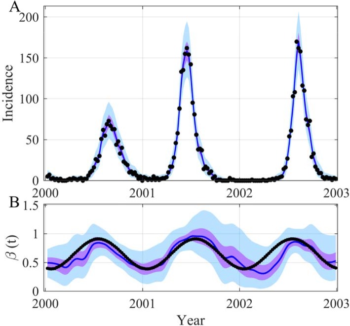
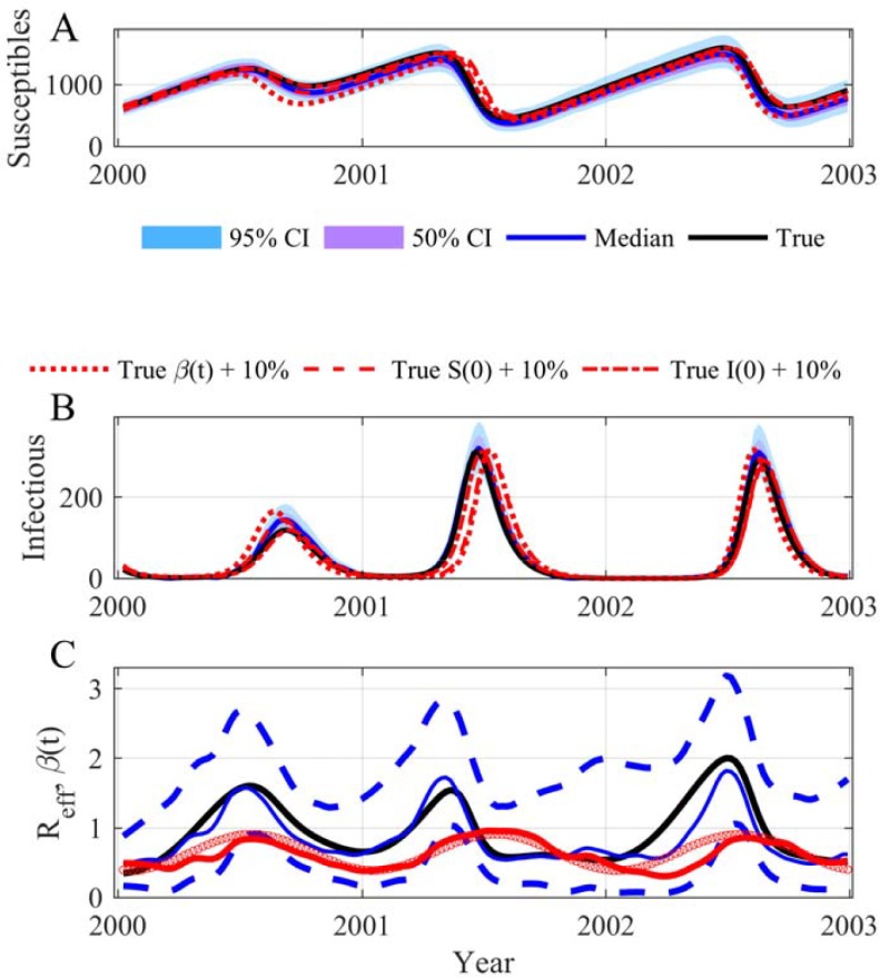
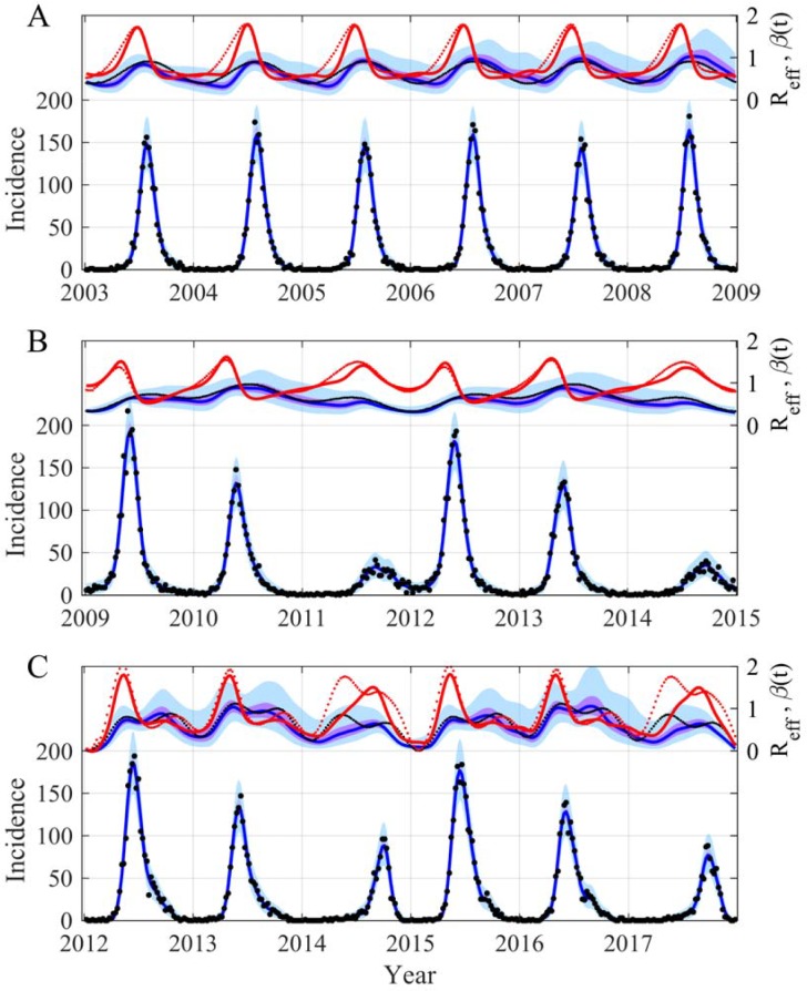
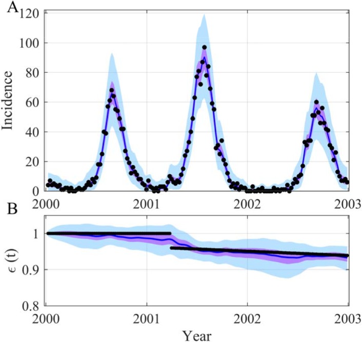
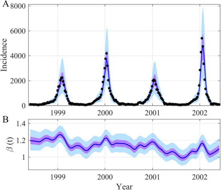
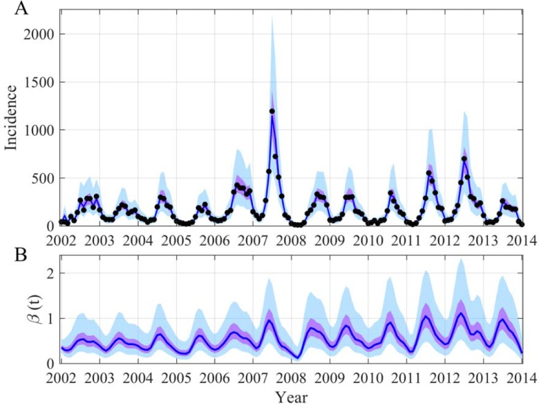
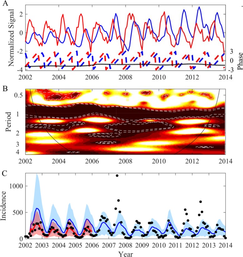
The spread of disease through human populations is complex. The characteristics of disease propagation evolve with time, as a result of a multitude of environmental and anthropic factors, this non-stationarity is a key factor in this huge complexity. In the absence of appropriate external data sources, to correctly describe the disease propagation, we explore a flexible approach, based on stochastic models for the disease dynamics, and on diffusion processes for the parameter dynamics. Using such a diffusion process has the advantage of not requiring a specific mathematical function for the parameter dynamics. Coupled with particle MCMC, this approach allows us to reconstruct the time evolution of some key parameters (average transmission rate for instance). Thus, by capturing the time-varying nature of the different mechanisms involved in disease propagation, the epidemic can be described. Firstly we demonstrate the efficiency of this methodology on a toy model, where the parameters and the observation process are known. Applied then to real datasets, our methodology is able, based solely on simple stochastic models, to reconstruct complex epidemics, such as flu or dengue, over long time periods. Hence we demonstrate that time-varying parameters can improve the accuracy of model performances, and we suggest that our methodology can be used as a first step towards a better understanding of a complex epidemic, in situation where data is limited and/or uncertain.

Fig 1

Reconstruction of both the incidence (A) and the time evolution β(t) (B) for the SIRS model. In (A) the black points are observations generated with a Poisson process with a mean equal to the incidence simulated by the model. In (B) the black points are the true values of β(t) = β₀.(1 + β₁ sin(2π t/365+2πϕ)). The blue lines are the median of the posterior, the mauve areas are the 50% Credible Intervals (CI) and the light blue areas the 95% CI. For all the figures, the observation process is also applied to the inferred incidence trajectory. The time unit of the model is day, the initial date is arbitrary (2000-01-09) and parameters used for the SIRS model are as follows: μ = 1/(50*365), α = 1/(7*365), γ = 1/14, β₀ = 0.65, β₁ = 0.4, ϕ = -0.2, ρ = 1, N = 10000, S(0) = 600, I(0) = 30. The prior and posterior distributions of the inferred parameters are in S1 Fig.

Fig 2

Simulation of the SIRS model: (A) Susceptibles; (B) Infectious; (C) Time evolution of both R_eff and β(t). In (A) and (B) the black lines are the true values, the blue lines are the median of the posterior, the mauve areas are the 50% CI and the light blue areas the 95% CI. In (A) and (B) the susceptibles and infectious trajectories with a modification of 10% of the value of S(0), I(0) and β(t) have been added to show the weak sensitivity of the SIRS model to these values. In (C) the black line is the true values of R_eff, the blue line is the median of the posterior, and the dashed lines the 95% CI of R_eff; the red dot line is the true time evolution of β(t) and the red line the median of its posterior. Model parameters as in Fig 1: The time unit of the model is day, the initial date is arbitrary (2000-01-09) and parameters used for the SIRS model are the following: μ = 1/(50*365), α = 1/(7*365), γ = 1/14, β₀ = 0.65, β₁ = 0.4, ϕ = -0.2, ρ = 1, N = 10000, S(0) = 600, I(0) = 30.

Fig 3

Reconstruction of both the incidence (bottom panel) and the time evolution of β(t) and R_eff (top panel) for a SIRS model with the initial conditions near the attractor of the dynamics. The true β is generated by β(t) = β₀.(1 + β₁ sin(2π t/365+2πϕ) + β₂ sin(2πt/(3 365)+2πϕ))+ β₃ sin(2πt/(0.5 365)+2πϕ)) with in (A) β₁ = 0.4, β₂ = 0, β₃ = 0, S(0) = 911.5, I(0) = 3.5; in (B) β₁ = 0.4, β₂ = 0.3, β₃ = 0, S(0) = 1735, I(0) = 20; and in (C) β₁ = 0.1, β₂ = 0.1, β₃ = 0.1, S(0) = 3365, I(0) = 3. The other parameters used are as follows: μ = 1/(50*365), α = 1/(7*365), γ = 1/14, β₀ = 0.65, ϕ = -0.2, ρ = 1, N = 10000. In both panels blue lines are the median of the posterior, the mauve areas are the 50% CI and the light blue areas the 95% CI. In the top panel, the red line is the reconstructed R_eff, the points are the true values of R_eff (red) and of β(t) (black). In the bottom panel the black points are observations generated with a Poisson process. The prior and posterior distributions of the inferred parameters are in S3 Fig.

Fig 4

Reconstruction of both the incidence (A) and the time evolution of ε_S(t) (B) for the SIRS model. In (A) the black points are observations generated with a Poisson process with a mean equal to the incidence simulated by the model. In (B) the black points are the true value of ε_S(t): ε_S(t) = 1 and shift to ε_S(t) = 0.96 - (0.012/365)*(t—t_shift) at t_shift = 450 days after t₀ in days. The blue lines are the median of the posterior, the mauve areas are the 50% CI and the light blue areas the 95% CI. The time unit of the model is day, the initial date is arbitrary (2000-01-09), β(t) = β₀.(1 + β₁ sin(2πt/365+2πϕ)) and parameters used for the SIRS model are as follows: μ = 1/(50*365), α = 1/(7*365), γ = 1/14, β₀ = 0.65, β₁ = 0.4, ϕ = -0.2, ρ = 1, N = 10000, S(0) = 600, I(0) = 30. The prior and posterior distributions of the inferred parameters are in S15 Fig.

Fig 5

Reconstruction of both the incidence (A) and the time evolution β(t) (B) in the case of the 1998–2002 seasonal flu epidemics in Israel. In (A) the black points are influenza-like illness incidence collected by Israel’s Maccabi health maintenance organization [46]. The blue lines are the median of the posterior, the mauve areas are the 50% CI and the light blue areas the 95% CI. The prior and posterior distributions of the inferred parameters are in S16 Fig.

Fig 6

Reconstruction of both the incidence (A) and the time evolution of β(t) (B) in the case of the 2002–2013 dengue epidemics in the province of Phnom Penh (Cambodia). In (A) the black points are dengue incidence recorded by the Cambodian National surveillance (National Dengue Control Program from the Ministry of Health, see [47]). The blue lines are the median of the posterior, the mauve areas are the 50% CI and the light blue areas the 95% CI. The prior and posterior distributions of the inferred parameters are in S17 Fig.

Fig 7. Association between dengue transmission rate and monthly average maximum temperature in the province of Phnom Penh (Cambodia).

(A) Time evolution of the normalized median of β(t) (blue line) and average temperature (red line) as well as the evolution of their phase computed based on wavelet decomposition (see Method and [48,70]), blue dashed line for the normalized β(t), red dashed line for the normalized averaged temperature and black dotted line for their phase difference. (B) Wavelet coherence (see Method and [48,70]) between the reconstructed β(t) and average temperature. The colors code for low values in white to high values in dark red. The white dashed lines show the 90% and the 95% CI computed with adapted bootstrappes [71]. (C) Model simulations using a linear model describing β(t) with monthly average maximum temperature (S18 Fig) and monthly average minimum temperature (S19 Fig) (β(t) = a₀ + a₁.MaxTemp(t)+a₂.MinTemp(t)). The red line is the median of the posterior and the red area is the 95% CI when parameters are estimated for the period 2002–2005. The blue line is the median of the posterior and the light blue area is the 95% CI when parameters are estimated for the full time period. The black points are dengue incidence recorded by the Cambodian National surveillance [47].