. 2018 Jun 13;5(6):171628.
doi: 10.1098/rsos.171628. eCollection 2018 Jun.

Forward and inverse problems in the mechanics of soft filaments

Affiliations

Forward and inverse problems in the mechanics of soft filaments

M Gazzola et al. R Soc Open Sci. .

Abstract

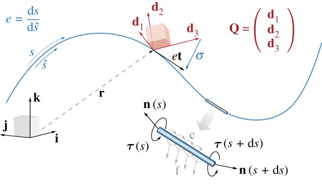
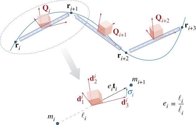
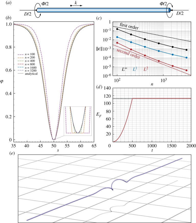
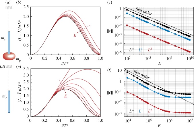
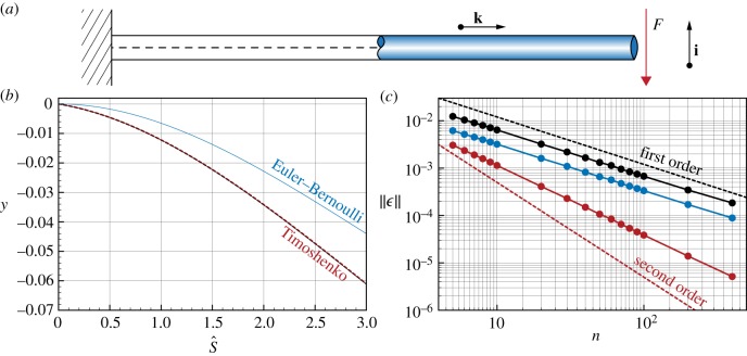
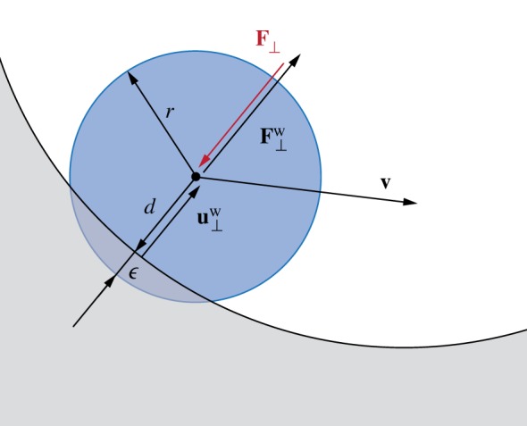
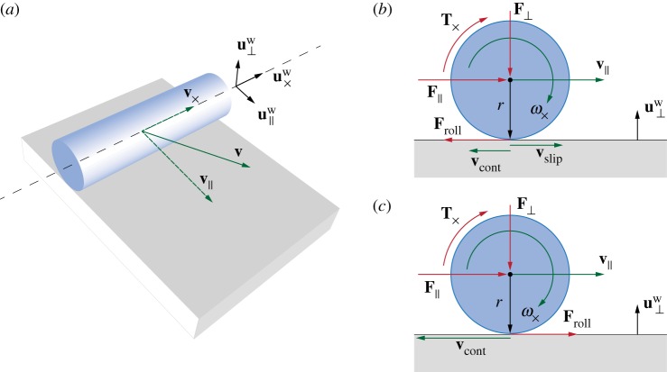
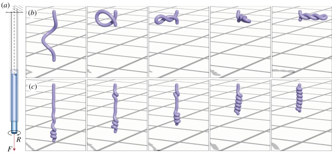
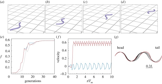
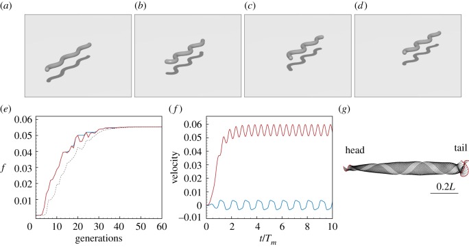
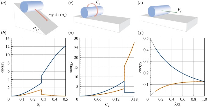
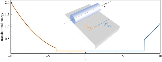
Soft slender structures are ubiquitous in natural and artificial systems, in active and passive settings and across scales, from polymers and flagella, to snakes and space tethers. In this paper, we demonstrate the use of a simple and practical numerical implementation based on the Cosserat rod model to simulate the dynamics of filaments that can bend, twist, stretch and shear while interacting with complex environments via muscular activity, surface contact, friction and hydrodynamics. We validate our simulations by solving a number of forward problems involving the mechanics of passive filaments and comparing them with known analytical results, and extend them to study instabilities in stretched and twisted filaments that form solenoidal and plectonemic structures. We then study active filaments such as snakes and other slender organisms by solving inverse problems to identify optimal gaits for limbless locomotion on solid surfaces and in bulk liquids.

Keywords: Cosserat theory; computational mechanics; soft filaments.


Conflict of interest statement

The authors declare no competing interests.

Figures

Figure 1.
Figure 1.
The Cosserat rod model. A filament deforming in the three-dimensional space is represented by a centre-line coordinate r and a material frame characterized by the orthonormal triad {d1,d2,d3}. The corresponding orthogonal rotation matrix Q with row entries d1, d2, d3 transforms a vector x from the laboratory canonical basis {i,j,k} to the material frame of reference {d1,d2,d3} so that xL=Qx and vice versa x=QTxL. If extension or compression is allowed, the current filament configuration arc-length s may no longer coincide with the rest reference arc-length s^. This is captured via the scalar dilatation field e=ds/ds^. Moreover, to account for shear we allow the triad {d1,d2,d3} to detach from the unit tangent vector t so that d3t (we recall that the condition d3=t and e=1 correspond to the Kirchhoff constraint for unshearable and inextensible rods, and implies that σ=etd3=0). The dynamics of the centre line and the material frame is determined at each cross section by the internal force and torque resultants, n and τ. External loads are represented via the force f and couple c line densities.
Figure 2.
Figure 2.
Discretization model. A discrete filament is represented through a set of vertices r(t)i=1,…,N+1 and a set of material frames Qi(t)={d1i,d2i,d3i,}i=1,,N. Two consecutive vertices define an edge of length ℓi along the tangent unit vector ti. The dilatation is defined as ei=i/^i, where ^i is the edge rest length. The vector σi=eitid3i represents the discrete shear and axial strains. The mass mr of the filament is discretized in pointwise concentrated masses mi=1,,n+1 at the locations ri for the purpose of advecting the vertices in time. For the evolution of Qi in time, we consider instead the mass second moment of inertia J^i=1,,n associated with the cylindrical elements depicted in blue.
Figure 3.
Figure 3.
Time–space convergence study for localized helical buckling. (a) We consider a rod originally straight whose ends are pulled together in the axial direction k with a slack D/2 and simultaneously twisted by the angle Φ/2. (b) Comparison between the analytical envelope function φ(s) and numerical approximations φn(s) at different levels of time–space resolution. Here, the time discretization δt is slaved by the spatial discretization δl=L/n according to δt=10−3δl s. (c) Norms L(ϵ) (black), L1(ϵ) (blue) and L2(ϵ) (red) are plotted against the number of discretization elements n. (d) Time evolution of the total energy of a rod (n=800, here the energy is computed assuming quadratic functionals, a suitable representation for an inextensible rod) simulated assuming no dissipation γ=0 (red line) versus the theoretical total energy EF=(MhΦ+ ThD)/2 (black dashed line). (e) Equilibrium rod configuration reqn numerically obtained given the discretization n=800, and assuming dissipation. For all studies, unless specified otherwise, we used the following settings: length L= 100 m, twist Φ=27⋅2π, slack D=3 m, linear mass density ρ= 1 kg m−1, bending stiffness α=1.345 Nm2, twisting stiffness β=0.789 Nm2, shear/stretch matrix S=105⋅1 N, bend/twist matrix B=diag(α,α,β) Nm2, dissipation constant γ= 10−2 kg (ms)−1, radius r=0.35 m, twisting time Ttwist=500 s, relaxation time Trelax=104 s.
Figure 4.
Figure 4.
Vertical oscillation under gravity. (a,d) We consider a vertical rod of mass mr clamped at the top and with a mass mp attached to the free end. Assuming that the rod is stiff enough (i.e. kA^E=const), it oscillates due to gravity around the equilibrium position L^+ΔL, where ΔL*=g(mp+mr/2)/k with a period T=2π(mp+mr/ξ)/k with ξ≃3 for mpmr, and ξπ2/4 for mpmr. Therefore, the rod oscillates according to L(t)=L^+[1+sin(2πt/Tπ/2)]ΔL. (ab) Case mpmr with mp=100 kg and mr=1 kg. (b) By increasing the stiffness E=107, 2×10⁷, 3×10⁷, 5×10⁷, 108, 1010 Pa, the simulated oscillations (red lines) approach the analytical solution (dashed black line). (c) Convergence to the analytical solution in the norms L(ϵ) (black), L1(ϵ) (blue) and L2(ϵ) (red) with ϵ=∥L(t)−LE(t)∥, where LE is the length numerically obtained as a function of E. (cd) Case mpmr with mp=0 kg and mr=1 kg. (e) By increasing the stiffness E=104, 2×10⁴, 3×10⁴, 5×10⁴, 105, 2×10⁵, 109 Pa, the simulated oscillations approach the analytical solution. (f) Convergence to the analytical solution in the norms L(ϵ), L1(ϵ) and L2(ϵ) as a function of E. For all studies, we used the following settings: gravity g=9.81 m s−2, rod density ρ=103 kg m−3, shear modulus G=2E/3 Pa, shear/stretch matrix S^=diag(4GA^/3,4GA^/3,EA^)N, bend/twist matrix B^=diag(EI^1,EI^2,GI^3)Nm2, rest length L^=1m, rest cross-sectional area A^=mr/(L^ρ)m2, number of discretization elements n=100, timestep δt=T*/106, dissipation constant γ=0.
Figure 5.
Figure 5.
Time–space convergence study for a cantilever beam. (a) We consider the static solution of a beam clamped at one end s^=0 and subject to the downward force F at the free end s^=L^. (b) Comparison between the Timoshenko analytical y (black lines) and numerical yn (with n=400, red dashed lines) vertical displacements with respect to the initial rod configuration. As a reference we report in blue the corresponding Euler–Bernoulli solution. (c) Norms L(ϵ) (black), L1(ϵ) (blue) and L2(ϵ) (red) of the error ϵ=∥yyn∥ at different levels of time–space resolution are plotted against the number of discretization elements n. Here, the time discretization δt is slaved by the spatial discretization n according to δt=10−2δl seconds. For all studies, we used the following settings: rod density ρ=5000 kg m−3, Young’s modulus E=106 Pa, shear modulus G=104 Pa, shear/stretch matrix S^=diag(4GA^/3,4GA^/3,EA^)N, bend/twist matrix B^=diag(EI^1,EI^2,GI^3)Nm2, downward force F=15 N, rest length L^=3m, rest radius r^=0.25m, dissipation constant γ=10−1 kg (ms)−1, simulation time Tsim=5000 s.
Figure 6.
Figure 6.
Muscular activity. Example of muscular activity amplitude profile (solid black line) described by cubic B-spline through Nm=8 control points (S^i,βi) with i=0,…,Nm−1. The control points are located along the filament at the positions S^i, and are associated with the amplitude values βi. The first and last control points are fixed so that (S^0,β0)=(0,0) and (S^Nm1,βNm1)=(L^,0), therefore assuming the ends of the deforming body to be free.
Figure 7.
Figure 7.
Contact model with solid boundaries. Obstacles and surfaces (grey) are modelled as soft boundaries allowing for the interpenetration ϵ=rd with the elements of the filament (blue) characterized by radius r and distance d from the substrate. The surface normal uw determines the direction of the wall’s response Fw to contact. We note that Fw balances the sum of all forces F that push the rod against the wall, and is complemented by the other two components, which allow it to amend to possible interpenetration due to numerics. These components are an elastic one (kwϵ) and a dissipative one (γwvuw), where kw and γw are, respectively, the wall stiffness and dissipation coefficients.
Figure 8.
Figure 8.
Surface friction. (a) The forces produced by friction effects between an element of the rod and the substrate are naturally decomposed into a lateral component in the direction uw=t×uw and a longitudinal one in the direction u×w=uw×uw. We note that in general uw×t. The notation x, x, x× denotes the projection of the vector x in the directions uw, uw, uw×. (b,c) Kinematic and dynamic quantities at play at any cross section in the case of (b) rolling and slipping and (c) pure rolling motion. Red arrows correspond to forces and torques, green arrows correspond to velocities, and black arrows correspond to geometric quantities.
Figure 9.
Figure 9.
Formation of plectonemes and solenoids. (a) We consider a soft rod clamped at one end, subject to a constant vertical load F and twisted R times at the other end. (b) Formation of a plectoneme for F=0 (leading to the total elongation L/L^1) and R=4. (c) Formation of a solenoid for F=300 N (leading to the total elongation L/L^1.15) and R=13. Settings: length L=1 m, radius r=0.025 m, mass m=1 kg, Young’s modulus E= 106 Pa, shear modulus G=2E/3 Pa, shear/stretch matrix S^=diag(4GA^/3,4GA^/3,EA^)N, bend/twist matrix B^=diag(EI1,EI2,GI3)Nm2, dissipation constant γ=2 kg (ms)−1, ksc= 104 kg s−2, γsc=10 kg s−1, discretization elements n=100, timestep δt=0.01δl s, Ttwist=75 s, Trelax= 50 s.
Figure 10.
Figure 10.
Optimal lateral undulation gait. (ad) Instances at different times of a snake characterized by the identified optimal gait. (e) Evolution of the fitness function f=vfwdmax as a function of the number of generations produced by CMA-ES. Solid blue, solid red and dashed black lines represent, respectively, the evolution of f corresponding to the best solution, the best solution within the current generation, and the mean generation value. (f) Scaled forward (red) and lateral (blue) centre of mass velocities versus normalized time. (g) Gait envelope over one oscillation period Tm. Red lines represent head and tail displacement in time. Settings: Froude number Fr=0.1, length L=1 m, radius r= 0.025 m, density ρ=103 kg m−3, Tm=1 s, Young’s modulus E=107 Pa, shear modulus G=2E/3 Pa, shear/stretch matrix S^=diag(4GA^/3,4GA^/3,EA^) N, bend/twist matrix B^=diag(EI1,EI2,GI3)Nm2, dissipation constant γ= 5 kg (ms)−1, gravity g=9.81 m s−2, friction coefficient ratios μkf:μkb:μkr=1:1.5:2 and μsf:μsb:μsr=1:1.5:2 with μsf=2μkf, friction threshold velocity vϵ=108ms1, ground stiffness and viscous dissipation kw=1 kg s−2 and γw=10−6 kg s−1, discretization elements n=50, timestep δt=2.5⋅10−5 Tm, wavelength λm=0.97L, phase shift ϕm=0, torque B-spline coefficients βi=0,…,5={0,17.4,48.5,5.4,14.7,0} Nm, bounds maximum attainable torque |β|maxi=0,…,5=50 Nm.
Figure 11.
Figure 11.
Optimal planar swimming gait at low Reynolds number. (ad) Instances at different times of a filament swimming according to the identified optimal gait. (e) Evolution of the fitness function f=vfwdmax as a function of the number of generations produced by CMA-ES. Solid blue, solid red and dashed black lines represent, respectively, the evolution of f corresponding to the best solution, the best solution within the current generation, and the mean generation value. (f) Scaled forward (red) and lateral (blue) centre of mass velocities versus normalized time. (g) Gait envelope over one oscillation period Tm. Red lines represent head and tail displacement in time. Settings: Reynolds number Re=10−4, length L=1 m, radius r=0.025 m, filament density ρ=103 kg m−3, Tm=1 s, Young’s modulus E=107 Pa, shear modulus G=2E/3 Pa, shear/stretch matrix S^=diag(4GA^/3,4GA^/3,EA^) N, bend/twist matrix B^=diag(EI1,EI2,GI3)Nm2, dissipation constant γ=5 kg (ms)−1, discretization elements n=50, timestep δt=2.5×10⁻⁵ Tm, wavelength λm=2.6L, phase shift ϕm=0, torque B-spline coefficients βi=0,…,5={0,50,50,50,50,0} Nm, bounds maximum attainable torque |β|maxi=0,…,5=50 Nm.
Figure 12.
Figure 12.
Comparison with hyperelastic models. Load response in a stretched rubber beam for different models.
Figure 13.
Figure 13.
Free body diagram of an infinitesimal beam element. The sketch represents an infinitesimal element undergoing bending and shear deformations, assuming small deflections so that xs. The bending moment is denoted as M, the shear force as V , the vertical displacement as y. The bending angle ψ, the shear angle θ and the slope of the vertical displacement dxy are related to each other so that ψ=θ+dxy.
Figure 14.
Figure 14.
Euler buckling instability. (a) Inextensible and unshearable rod vertically initialized and subject to the axial load F. (b) Probability P of observing an instability event as a function of the compression force F and the bending rigidity α for a fixed length L=1 m. The corresponding analytical solution is overlaid as reference (white line). (c) Probability P of observing an instability event as a function of the compression force F and the length L for a fixed bending rigidity α=1 Nm2. The corresponding analytical solution is overlaid as reference (white line). The probability P is determined by performing 10 simulations for each pair of parameters (F,α) or (F,L). Each simulation is initially perturbed by applying to every discretization node a small random force sampled from a uniform distribution, such that FRU(0,102)N. The occurrence of an instability is detected whenever the rod bending energy EB>Eth with Eth=10−3 J. Settings: rod’s mass mr=1 kg, twist stiffness β=2α/3 Nm2, shear/stretch matrix S=105×1 N, bend/twist matrix B=diag(α,α,β) Nm2, radius r=0.025L m, discretization elements n=100 m−1, timestep δt= 10−5 s, simulation time Tsim=10 s, dissipation constant γ=0.
Figure 15.
Figure 15.
Mitchell buckling instability. (a) Probability P of observing an instability event as a function of the total twist Φ and the ratio between bending and twist rigidities β/α. The corresponding analytical solution is overlaid as reference (white line). The probability P is determined by performing 10 simulations for each pair of parameters (Φ,β/α). Each simulation is initially perturbed by applying to every discretization node a small random force sampled from a uniform distribution, such that FRU(0,103)N. The occurrence of an instability is detected whenever the rod translational energy ET>Eth with Eth=10−4 J. (bc) Visualization of a Mitchell bucking instability event for Φ=10 and β/α=2. Settings: rod’s mass mr=1 kg, length L= 1 m, bending stiffness α=1 Nm2, shear/stretch matrix S= 105×1 N, bend/twist matrix B=diag(α,α,β) Nm2, radius r= 0.01L m, discretization elements n=50 m−1, timestep δt= 10−5 s, simulation time Tsim=2 s, dissipation constant γ=0.
Figure 16.
Figure 16.
Time-space convergence study for twist forced vibrations in a stretched rod. (a) We consider a rod clamped at one end, forced to vibrate by applying the periodic couple Avsin(2πfvt) to the free end, and characterized by rest length L^ which is extended to a final length L=eL^. (b) Comparison between analytical θ (black lines) and numerical θn (red dashed lines) angular displacement with respect to the reference configuration along a stretched rod. Each red (numerical simulation) and black (analytical solution) line corresponds to the angular displacement along a rod discretized with n=1600 elements, and sampled at regular intervals Δt=Tv/10 within one loading period Tv=fv1. (c) Norms L(ϵ) (black), L1(ϵ) (blue) and L2(ϵ) (red) of the error ϵ=∥θθn∥ at different levels of time-space resolution are plotted against the number of discretization elements n. Here, the time discretization δt is slaved by the spatial discretization n according to δt=10−4δl seconds. For all studies, we used the following settings: rod’s density ρ=10 kg m−3, Young’s modulus E=106 Pa, shear modulus G=2E/3 Pa, shear/stretch matrix S^=diag(4GA^/3,4GA^/3,EA^)N, bend/twist matrix B^=diag(EI^1,EI^2,GI^3)Nm2, forcing amplitude Av=103 Nm, forcing frequency fv=1 s−1, dilatation factor e=1.05, rest length L^=E/ρ/(efv)m, rest radius r^=0.5m, simulation time Tsim=2000 s. We enabled dissipation in the early stages of the simulations, letting γ decay exponentially in time to a zero value.
Figure 17.
Figure 17.
Rolling static and dynamic friction. (a) A rod initially at rest on a plane inclined of the angle αs rolls or slips down with linear and angular velocities v and ω due to its own weight mg. (b) Translational ET=mv2/2 (analytical solution: black line, numerical solution: blue line) and rotational ER=2/2 (analytical solution: dashed black line, numerical solution: orange line) energies are plotted against the angle αs. Settings: length L=1 m, radius r= 0.025 m, mass m=1 kg, Young’s modulus E=109 Pa, shear modulus G=2E/3 Pa, shear/stretch matrix S=104×1 N, bend/twist matrix B=diag(EI1,EI2,GI3) Nm2, dissipation constant γ=10−6 kg (ms)−1, gravity g=9.81 m s−2, static and kinetic friction coefficients μs=0.4 and μk=0.2, friction threshold velocity vϵ=104ms1, ground stiffness and viscous dissipation kw=10 kg s−2 and γw=10−4 kg s−1, discretization elements n=50, timestep δt= 10−6 s, simulation time T=0.5 s. (c) Rod set in motion by the external couple Cs on a horizontal plane. (d) Translational ET and rotational ER energies are plotted against the couple Cs. Colour scheme and settings are identical to those of panel (b) except for the simulation time T=1 s. (e) Rod with initial velocity V s slows down due to kinetic friction until the no slip condition is reached. (f) Translational ET and rotational ER energies are plotted against the relative mass moment of inertia ratio λ/2. Colour scheme and settings are identical to those of (b) except for the simulation time T=2 s, and the friction threshold velocity vϵ=10−6 m s−1.
Figure 18.
Figure 18.
Anisotropic static and kinetic longitudinal friction. A rod initially at rest on a horizontal plane is pulled longitudinally with force F. The system is characterized by anisotropic friction so that resistance forces in the forward direction Fflong are larger than in the backward direction Fblong. The plot illustrates the behaviour of the total rod’s translational energy ET as a function of the force F applied. Blue and solid black lines correspond to, respectively, simulated and analytical ET for a rod pulled forward. Orange and dashed black lines correspond to, respectively, simulated and analytical ET for a rod pulled backward. Settings: length L=1 m, radius r= 0.025 m, mass m=1 kg, Young’s modulus E=105 Pa, shear modulus G=2E/3 Pa, shear/stretch matrix S=104×1 N, bend/twist matrix B=diag(EI1,EI2,GI3) Nm2, dissipation constant γ=10−6 kg (ms)−1, gravity g=9.81 m s−2, static and kinetic forward friction coefficients μfs=0.8 and μfk=0.4, static and kinetic backward friction coefficients μbs=0.4 and μbk=0.2, friction threshold velocity vϵ=104ms1, ground stiffness and viscous dissipation kw=10 kg s−2 and γw=10−4 kg s−1, discretization elements n=50, timestep δt=10−5 s, simulation time T=0.25 s.
Figure 19.
Figure 19.
Isotropic versus anisotropic friction driven locomotion. (a) Gait envelope computed over the 10th muscular activation cycle in the case of isotropic friction. The blue triangle denotes the location of the snake’s centre of mass at time t=0, reported as reference. (b) Lateral (blue) and forward (red) velocities as functions of time normalized by the activation period Tm in the case of isotropic friction. (c) Gait envelope computed over the 10th muscular activation cycle in the case of anisotropic friction. The blue triangle denotes the location of the snake’s centre of mass at time t=0, reported as reference. (d) Lateral (blue) and forward (red) velocities as functions of time normalized by the activation period Tm in the case of anisotropic friction. Settings: length L=0.5 m, radius r= 0.025 m, mass m=1 kg, Young’s modulus E=107 Pa, shear modulus G=2E/3 Pa, shear/stretch matrix S=105×1 N, bend/twist matrix B=diag(EI1,EI2,GI3) Nm2, dissipation constant γ= 10−1 kg (ms)−1, gravity g=9.81 m s−2, static μfs=0.2, μsr=μsf, μsb=μsf and kinetic μfk=0.1, μkr=μkf, μkb=μkf friction coefficients in the isotropic case, static μfs=0.2, μsr=2μsf, μsb=20μsf and kinetic μfk= 0.1, μkr=2μkf, μkb=20μkf friction coefficients in the anisotropic case, friction threshold velocity vϵ=108ms1, ground stiffness and viscous dissipation kw=1 kg s−2 and γw=10−6 kg s−1, discretization elements n=100, timestep δt= 10−5 s, muscular activation period Tm=1 s, wavelength λm=, phase shift ϕm=0, torque B-spline coefficients βi=0,…,5={0,10,15,15,10,0} Nm.
Figure 20.
Figure 20.
Timings for various representative simulations. The time-to-solution values reported correspond to an average over 10 measurements for the same study case.

Similar articles

Cited by

References

    1. Kirchhoff G. 1859. Ueber das gleichgewicht und die bewegung eines unendlich dünnen elastischen stabes. J. Reine Angew. Math. 56, 285–313. (doi:10.1515/crll.1859.56.285) - DOI
    1. Clebsch A. 1883. Théorie de l’élasticité des corps solides. Paris, France: Dunod.
    1. Love AEH. 1906. A treatise on the mathematical theory of elasticity. Cambridge, UK: Cambridge University Press.
    1. Cosserat E, Cosserat F. 1909. Théorie des corps déformables. Ithaca, NY: Cornell University Library.
    1. Antman SS. 1973. The theory of rods. Berlin, Germany: Springer.

LinkOut - more resources