

Stochastic Hybrid Systems in Cellular Neuroscience
- PMID: 30136005
- PMCID: PMC6104574
- DOI: 10.1186/s13408-018-0067-7
Stochastic Hybrid Systems in Cellular Neuroscience
Abstract
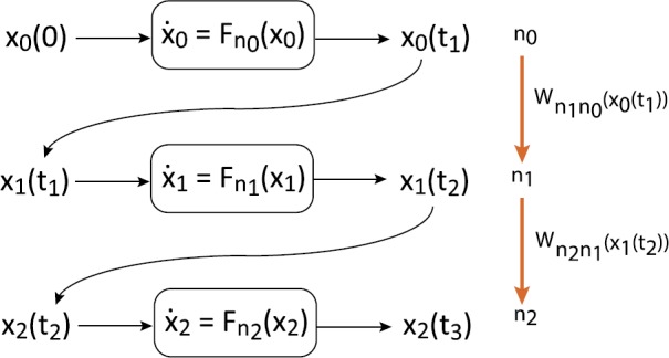
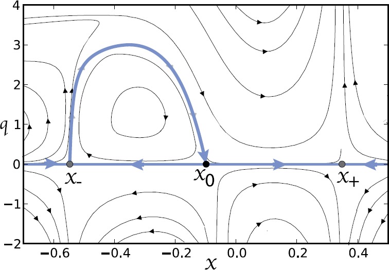
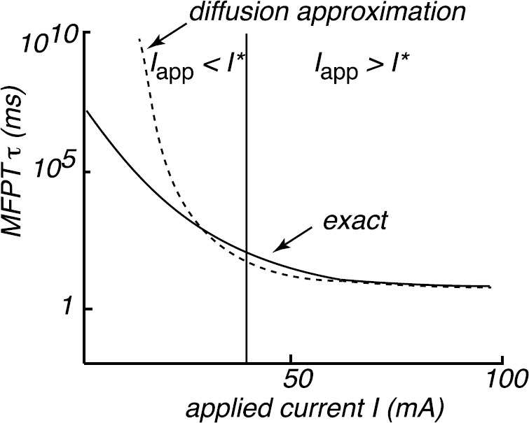
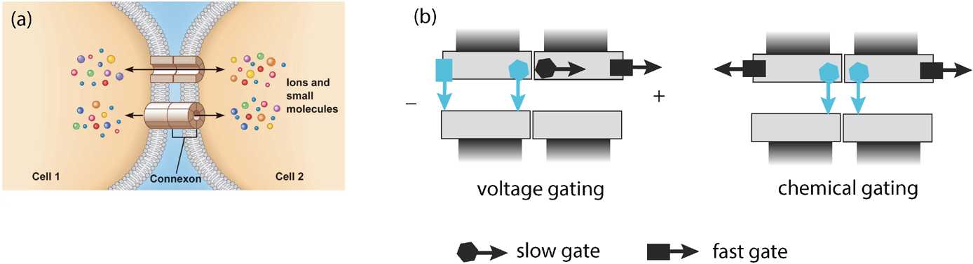
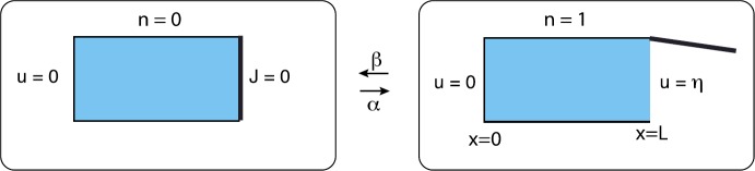
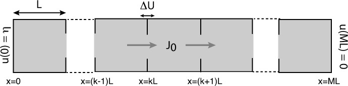
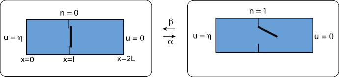
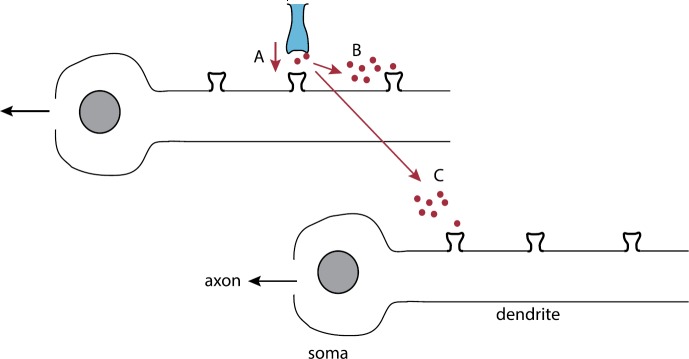
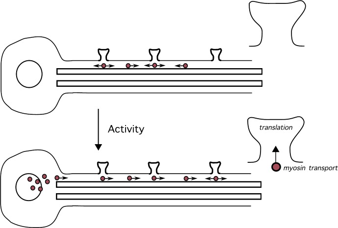
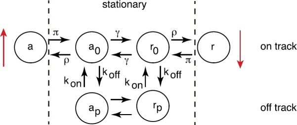
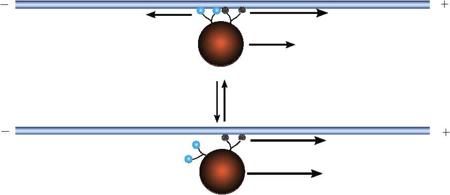
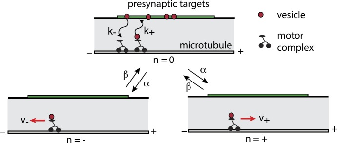
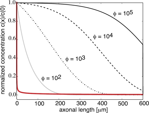
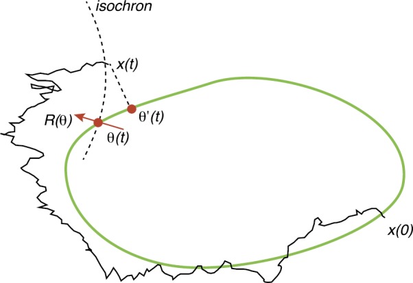
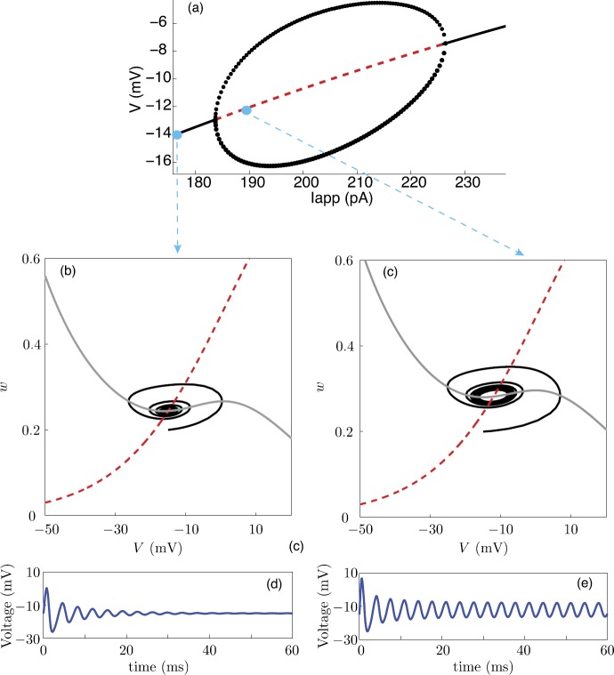
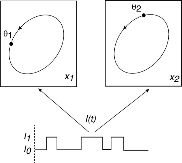
We review recent work on the theory and applications of stochastic hybrid systems in cellular neuroscience. A stochastic hybrid system or piecewise deterministic Markov process involves the coupling between a piecewise deterministic differential equation and a time-homogeneous Markov chain on some discrete space. The latter typically represents some random switching process. We begin by summarizing the basic theory of stochastic hybrid systems, including various approximation schemes in the fast switching (weak noise) limit. In subsequent sections, we consider various applications of stochastic hybrid systems, including stochastic ion channels and membrane voltage fluctuations, stochastic gap junctions and diffusion in randomly switching environments, and intracellular transport in axons and dendrites. Finally, we describe recent work on phase reduction methods for stochastic hybrid limit cycle oscillators.
Conflict of interest statement
Ethics approval and consent to participate
Not applicable.
Competing interests
The authors declare that they have no competing interests.
Consent for publication
Not applicable.
Figures

Similar articles
-
Synchronization of stochastic hybrid oscillators driven by a common switching environment.Chaos. 2018 Dec;28(12):123123. doi: 10.1063/1.5054795. Chaos. 2018. PMID: 30599535
-
Feynman-Kac formula for stochastic hybrid systems.Phys Rev E. 2017 Jan;95(1-1):012138. doi: 10.1103/PhysRevE.95.012138. Epub 2017 Jan 23. Phys Rev E. 2017. PMID: 28208495
-
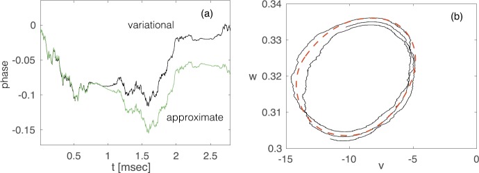
A variational method for analyzing limit cycle oscillations in stochastic hybrid systems.Chaos. 2018 Jun;28(6):063105. doi: 10.1063/1.5027077. Chaos. 2018. PMID: 29960393
-
Simulation Strategies for Calcium Microdomains and Calcium Noise.Adv Exp Med Biol. 2020;1131:771-797. doi: 10.1007/978-3-030-12457-1_31. Adv Exp Med Biol. 2020. PMID: 31646534 Review.
-
Simulation strategies for calcium microdomains and calcium-regulated calcium channels.Adv Exp Med Biol. 2012;740:553-67. doi: 10.1007/978-94-007-2888-2_25. Adv Exp Med Biol. 2012. PMID: 22453960 Review.
Cited by
-
Special Issue from the 2017 International Conference on Mathematical Neuroscience.J Math Neurosci. 2019 Jan 7;9(1):1. doi: 10.1186/s13408-018-0069-5. J Math Neurosci. 2019. PMID: 30617922 Free PMC article.
-
A Ca2+ puff model based on integrodifferential equations.J Math Biol. 2025 Mar 25;90(4):43. doi: 10.1007/s00285-025-02202-3. J Math Biol. 2025. PMID: 40131459 Free PMC article.
-
Modular architecture facilitates noise-driven control of synchrony in neuronal networks.Sci Adv. 2023 Aug 25;9(34):eade1755. doi: 10.1126/sciadv.ade1755. Epub 2023 Aug 25. Sci Adv. 2023. PMID: 37624893 Free PMC article.
References
-
- Alberts B, Johnson A, Lewis J, Raff M, Walter KR. Molecular biology of the cell. 5. New York: Garland; 2008.
-
- Anderson DF, Ermentrout GB, Thomas PJ. Stochastic representations of ion channel kinetics and exact stochastic simulation of neuronal dynamics. J Comput Neurosci. 2015;38:67–82. - PubMed
-
- Bakhtin Y, Hurth T, Lawley SD, Mattingly JC. Smooth invariant densities for random switching on the torus. Preprint. arXiv:1708.01390 (2017).
-
- Bena I. Dichotomous Markov noise: exact results for out-of-equilibrium systems. Int J Mod Phys B. 2006;20:2825–2888.
Publication types
Grants and funding
LinkOut - more resources
Full Text Sources
Other Literature Sources
Molecular Biology Databases
Miscellaneous
