Non-local Parabolic and Hyperbolic Models for Cell Polarisation in Heterogeneous Cancer Cell Populations

Abstract

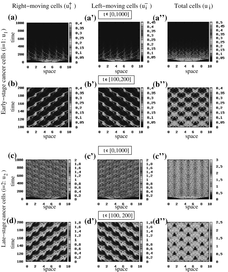
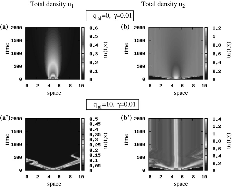
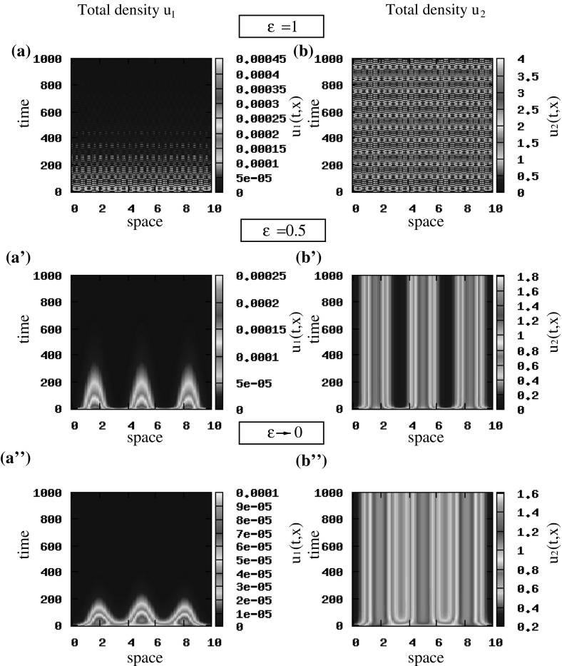
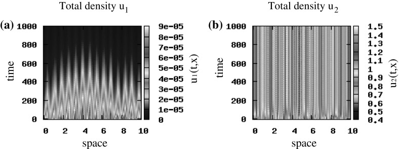
Tumours consist of heterogeneous populations of cells. The sub-populations can have different features, including cell motility, proliferation and metastatic potential. The interactions between clonal sub-populations are complex, from stable coexistence to dominant behaviours. The cell-cell interactions, i.e. attraction, repulsion and alignment, processes critical in cancer invasion and metastasis, can be influenced by the mutation of cancer cells. In this study, we develop a mathematical model describing cancer cell invasion and movement for two polarised cancer cell populations with different levels of mutation. We consider a system of non-local hyperbolic equations that incorporate cell-cell interactions in the speed and the turning behaviour of cancer cells, and take a formal parabolic limit to transform this model into a non-local parabolic model. We then investigate the possibility of aggregations to form, and perform numerical simulations for both hyperbolic and parabolic models, comparing the patterns obtained for these models.

Keywords: Aggregation patterns; Alignment; Cancer cells; Cell–cell interactions; Non-local hyperbolic model; Parabolic limit.

Fig. 1

The dispersion relation (21) for the steady state $\left(0,0,0,0\right)$. a Plot of the larger eigenvalues ${\lambda }_l\left(k\right)=\left(-D_l\left(k\right)+\sqrt{D_l^2\left(k\right)-4E_l\left(k\right)}\right)/2,l=1,2$, obtained by dispersion relations (21) for $D_1,E_1$ (blue) and $D_2,E_2$ (red); b the effect of $\gamma$ on the graph of $Re\left({\lambda }_2\left(k\right)\right)$; c the effect of $r_2$ on the graph of $Re\left({\lambda }_2\left(k\right)\right)$; d the effect of ${\lambda }_2^{\mathrm{r}}$ on the graph of $Re\left({\lambda }_2\left(k\right)\right)$. The continuous curves represent the $Re(\lambda (k))$, while the dotted curves represent the $Im(\lambda (k))$. The model parameters are given in Table 2. The diamonds on the x-axis represent the discrete wave numbers $k_j=2\pi j/L,j=1,2,\cdots$ (Color figure online)

Fig. 2

The dispersion relation (26) for the steady state $\left(0,0,0.5,0.5\right)$. a Plot of the larger eigenvalues ${\lambda }_l\left(k\right)=\left(-D_l\left(k\right)+\sqrt{D_l^2\left(k\right)-4E_l\left(k\right)}\right)/2,l=3,4$, obtained by dispersion relations (26) for $D_3,E_3$ (blue) and $D_4,E_4$ (red); b the effect of $\gamma$ on the graph of $Re\left({\lambda }_4\left(k\right)\right)$; c the effect of $r_2$ on the graph of $Re\left({\lambda }_4\left(k\right)\right)$; d the effect of ${\lambda }_2^{\mathrm{r}}$ on the graph of $Re\left({\lambda }_4\left(k\right)\right)$; e the effect of $q_{\mathrm{a}}$ on the graph of $Re\left({\lambda }_4\left(k\right)\right)$; f the effect of $q_{\mathrm{r}}$ on the graph of $Re\left({\lambda }_4\left(k\right)\right)$. The continuous curves represent the $Re(\lambda (k))$, while the dotted curves represent the $Im(\lambda (k))$. The model parameters are given in Table 2. The diamonds on the x-axis represent the discrete wave numbers $k_j=2\pi j/L,j=1,2,\cdots$ (Color figure online)

Fig. 3

Plot of the eigenvalue with the maximum real part, after parabolic scaling, of a relation (21) for the s.s. $\left(0,0,0,0\right)$ for $q_{\mathrm{al}}=0$; b relation (26) for the s.s. $\left(0,0,0.5,0.5\right)$ for $q_{\mathrm{al}}=0$. The continuous curves represent the $Re(\lambda (k))$, while the dotted curves represent the $Im(\lambda (k))$. The rest of the model parameters are given in Table 2. For graphical purposes, the discrete wave numbers has been omitted (Color figure online)

Fig. 4

Plot of the eigenvalues obtained by dispersion relation (31). a ${\lambda }_1\left(k\right)=-k^2{D}_{u_1}-M+r_1$ (blue) and ${\lambda }_2\left(k\right)=-k^2{D}_{u_2}+r_2$ (red) for the steady state $\left(0,0\right)$; b ${\lambda }_1\left(k\right)=-k^2{D}_{u_1}-M$ (blue) and ${\lambda }_2\left(k\right)=-k^2{D}_{u_2}+Y\left(k\right)\left({\lambda }_2^{\mathrm{b}}{f}^{\prime }\left(-2\right)/(2{\lambda }_2^{\mathrm{r}})-1\right)-r_2$ (red), for the steady state $\left(0,1\right)$. The model parameters are given in Table 2. The continuous curves represent the $Re\left(\lambda (k)\right)$, as the imaginary part of the eigenvalues is zero (represented by dotted lines) in the case of the parabolic model [see relations (31)–(33)]. The diamonds on the x-axis represent the discrete wave numbers $k_j=2\pi j/L,j=1,2,\cdots$ (Color figure online)

Fig. 5

The dispersion relation (31) for the steady state $\left(0,1\right)$. a The effect of ${\lambda }_2^{\mathrm{r}}$ on the graph of $Re\left({\lambda }_2\left(k\right)\right)$; b the effect of $q_{\mathrm{r}}$ on the graph of $Re\left({\lambda }_2\left(k\right)\right)$; the rest of the model parameters are given in Table 2. The diamonds on the x-axis represent the discrete wave numbers $k_j=2\pi j/L,j=1,2,\cdots$ (Color figure online)

Fig. 6

Patterns exhibited by the hyperbolic model (1). The initial conditions for the two cancer cell populations are described by small random perturbations of the steady state $\left(0,0,0,0\right)$ [see (34)]. a, b Total density of $u_1=u_1^{+}+u_1^{-}$ and $u_2=u_2^{+}+u_2^{-}$ for $r_1=0.1$ and $r_2=0.2$; a’, b’ total density of $u_1=u_1^{+}+u_1^{-}$ and $u_2=u_2^{+}+u_2^{-}$ for $r_1=0.3$ and $r_2=0.4$; a”, b” total density of $u_1=u_1^{+}+u_1^{-}$ and $u_2=u_2^{+}+u_2^{-}$ for $r_1=r_2=0.1$. The rest of model parameters are given in Table 2 (Color figure online)

Fig. 7

Patterns exhibited by the hyperbolic model (1). The initial conditions for the two cancer cell populations are described by small random perturbations of the steady state $\left(0,0,0,0\right)$ [see (34)]. a, b Total density of $u_1=u_1^{+}+u_1^{-}$ and $u_2=u_2^{+}+u_2^{-}$ for ${\lambda }_{1,2}^{\mathrm{r}}=0.2$ and $\gamma =0.1$; a’, b’ total density of $u_1=u_1^{+}+u_1^{-}$ and $u_2=u_2^{+}+u_2^{-}$ for ${\lambda }_{1,2}^{\mathrm{r}}=0.4$ and $\gamma =0.1$; a”, b” total density of $u_1=u_1^{+}+u_1^{-}$ and $u_2=u_2^{+}+u_2^{-}$ for ${\lambda }_{1,2}^{\mathrm{r}}=0.2$ and $\gamma =1$. The rest of model parameters are given in Table 2 (Color figure online)

Fig. 8

Patterns exhibited by the hyperbolic model (1). The initial conditions for the two cancer cell populations are described by small random perturbations of the steady state $\left(0,0,0.5,0.5\right)$ [see (34)]. a, b Total density of $u_1=u_1^{+}+u_1^{-}$ and $u_2=u_2^{+}+u_2^{-}$ for $q_{\mathrm{a}}=6,q_{\mathrm{r}}=0.1$ and $q_{\mathrm{al}}=3$; a’, b’ total density of $u_1=u_1^{+}+u_1^{-}$ and $u_2=u_2^{+}+u_2^{-}$ for $q_{\mathrm{a}}=1.2,q_{\mathrm{r}}=6.5$ and $q_{\mathrm{al}}=3$. The rest of model parameters are given in Table 2 (Color figure online)

Fig. 9

Patterns exhibited by the hyperbolic model (1) for $q_{\mathrm{al}}=0.5$ and ${\lambda }_{1,2}^{\mathrm{r}}=0.1$. The rest of model parameters as given in Table 2. The initial conditions for the two cancer cell populations consist of a rectangular pulse [see (35)]. a–d show the density of right-moving cancer cells $u_1^{+}$ (a, b) and $u_2^{+}$ (c, d). a’–d’ show the density of left-moving cancer cells $u_1^{-}$ (a’, b’) and $u_2^{-}$ (c’, d’). a”–d” show the total density of cancer cells $u_1$ (a”, b”) and $u_2$ (c”, d”) (Color figure online)

Fig. 10

Patterns exhibited by the hyperbolic model (1) showing the cancer cell density for $\gamma =0.01$. The initial conditions for the two cancer cell populations consist of a rectangular pulse [see (35)]. a, b Total density of $u_1$ and $u_2$ for $q_{\mathrm{al}}=0$; a’, b’ total density of $u_1$ and $u_2$ for $q_{\mathrm{al}}=10$. The rest of model parameters are given in Table 2 (Color figure online)

Fig. 11

The spatiotemporal patterns obtained with the hyperbolic model (1) for $q_{\mathrm{al}}=0$ after scaling, and the parabolic model (12). a, b Standing waves obtained by (1) after scaling for $ϵ=1$; a’, b’ stationary pulses obtained by (1) after scaling for $ϵ=0.5$; a”, b” stationary pulses obtained by (12) when $ϵ\to 0$. The initial conditions for the two cancer cell populations are described by small random perturbation of the steady state $\left(0,0,0.5,0.5\right)$, for the rescaled hyperbolic model, and $\left(0,1\right)$, for the parabolic model [see (34) and (36)]. The rest of model parameters are given in Table 2 (Color figure online)

Fig. 12

Patterns exhibited by the parabolic model (12). The initial conditions for the two cancer cell populations are described by small random perturbations of the steady state $\left(0,1\right)$ [see (36)]. Total density of $u_1$ and $u_2$ for $q_{\mathrm{a}}=6,q_{\mathrm{r}}=0.1$ and $q_{\mathrm{al}}=0$. The rest of the model parameters are given in Table 2 (Color figure online)

Fig. 13

Patterns exhibited by the parabolic model (12) showing the cancer cell density for $\gamma =0.01$. The initial conditions for the two cancer cell populations consist of a rectangular pulse [see (37)]. a, b Total density of $u_1$ and $u_2$ for $q_{\mathrm{a}}=1.2,q_{\mathrm{r}}=0.1$ and $q_{\mathrm{al}}=0$. The rest of model parameters are given in Table 2 (Color figure online)

References

1. Anderson ARA, Chaplain MAJ, Newman EL, Steele RJC, Thompson AM. Mathematical modelling of tumour invasion and metastasis. J Theor Med. 2000;2(2):129–154. doi: 10.1080/10273660008833042. - DOI
1. Angelini T, Hannezo E, Trepat X, Fredberg J, Weitz D. Cell migration driven by cooperative substrate deformation patterns. Phys Rev Lett. 2010;104(16):168104. doi: 10.1103/PhysRevLett.104.168104. - DOI - PMC - PubMed
1. Arboleda-Estudillo Y, Krieg M, Stühmer J, Licata NA, Muller DJ, Heisenberg CP. Movement directionality in collective migration of germ layer progenitors. Curr Biol. 2010;20(2):161–169. doi: 10.1016/j.cub.2009.11.036. - DOI - PubMed
1. Armstrong NJ, Painter KJ, Sherratt JA. A continuum approach to modelling cell–cell adhesion. J Theor Biol. 2006;243(1):98–113. doi: 10.1016/j.jtbi.2006.05.030. - DOI - PMC - PubMed
1. Bitsouni V, Chaplain MAJ, Eftimie R. Mathematical modelling of cancer invasion: the multiple roles of TGF-β pathway on tumour proliferation and cell adhesion. Math Models Methods Appl Sci. 2017;27(10):1929–1962. doi: 10.1142/S021820251750035X. - DOI
Publication types
MeSH terms
LinkOut - more resources