Phylogeny Estimation by Integration over Isolation with Migration Models

Abstract

Phylogeny estimation is difficult for closely related populations and species, especially if they have been exchanging genes. We present a hierarchical Bayesian, Markov-chain Monte Carlo method with a state space that includes all possible phylogenies in a full Isolation-with-Migration model framework. The method is based on a new type of genealogy augmentation called a "hidden genealogy" that enables efficient updating of the phylogeny. This is the first likelihood-based method to fully incorporate directional gene flow and genetic drift for estimation of a species or population phylogeny. Application to human hunter-gatherer populations from Africa revealed a clear phylogenetic history, with strong support for gene exchange with an unsampled ghost population, and relatively ancient divergence between a ghost population and modern human populations, consistent with human/archaic divergence. In contrast, a study of five chimpanzee populations reveals a clear phylogeny with several pairs of populations having exchanged DNA, but does not support a history with an unsampled ghost population.

Fig. 1.

Phylogenies and Hidden Genealogies. The upper left panel shows a hidden genealogy in an island model of 3 populations adjacent to a phylogeny in which species 1 and 2 are most closely related. The operation of overlaying the phylogeny on the hidden genealogy generates the genealogy shown within a phylogeny on the right side of the upper panel. This operation leave some migration events irrelevant (hidden) because they occur between two populations that are not present in the phylogeny at the time of the migration event. In the middle row the same kind of operation is shown, using the same hidden genealogy as in the top row, but with a different phylogeny that causes a different genealogy (note that the order in which the populations are listed changes in this phylogeny). A third example with the same hidden genealogy is shown in the lower panel.

Fig. 2.

Phylogeny estimation while varying splitting time and migration. (A) A 3 population model was examined as $t_{0,1}$ varies from 0 to 1, where $t_{2,(0,1)}=1$ and (2,(0,1)) is the true phylogeny. Means and standard errors of estimated posterior probabilities for each phylogeny for 50 data sets simulated under each $t_{0,1}$ value are shown on the left axis. The proportion of maximum a posteriori (MAP) trees (out of 50) that matched the tree is shown on the right axis. (B) A 3 population model with migration that tends to obscure the true phylogenic topology, (2,(0, 1)). Mean and standard error of estimated posterior probabilities (left axis) for each phylogeny for 50 data sets simulated under each of a range of $2N{m}_{1>2}\mathrm{ }$values. The proportion of MAP trees matching the true tree is on the right axis.

Fig. 3.

Phylogeny estimation with four populations and zero migration, while varying migration priors, numbers of loci, and use of hyperprior distributions. Means and standard errors are shown for posterior probabilities (left axis) of phylogenies for 50 data sets simulated for each number of loci under a fixed phylogenetic topology, ((0, 1)4,(2, 3)5)6 where the ancestor populations (4, 5, and 6) are ordered in time (i.e., populations 0 and 1 split most recently, followed by 2 and 3). In each panel the mean posterior probability is shown for the estimated posteriors for the true tree, the mean of the two most similar trees ((2,(3,(0, 1)4)5)6 and (3,(2,(0, 1)4)5)6), and the mean of all other trees. The proportion of MAP trees matching the true tree is on the right axis. (A) Migration rate priors have a $U[0,\mathrm{ }0.1]$ distribution. (B) Migration rate priors have a $U[0,\mathrm{ }1]$ distribution. Also shown for the true tree are results using a hyperprior distribution for drift hyperparameters of U[0, 20] and for migration hyperparameters U[0.0, 1.0].

Fig. 4.

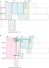
Estimated histories for human populations. Boxes represent populations, with widths proportional to estimated effective population sizes (ancestral $N_e$ is given for scale). Confidence intervals are indicated as dashed-line boxes aligned with the corresponding population’s box on the left side. Estimated population migration ($2N_{e}m$)rates that are associated with a migration rate significantly >0 based on a marginal likelihood ratio test (Nielsen and Wakeley 2001) are shown together with their estimated $2N_{e}m$ values (*$p<0.05$; **$p<0.01$; ***$p<0.001$) Migration rates not significantly different from zero at $p<0.01$ are not shown (a) Without a ghost population. Estimated splitting times are shown to scale with 95% confidence intervals. No migration rates were significantly different from zero. (b) With a ghost population. Splitting times are shown evenly distributed because of the great depth of the first split. The 95% confidence intervals for three recent splits are similar to part figure “a”. Confidence interval for the oldest split was 554–1,663 KYA.

Fig. 5.

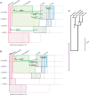
Estimated phylogenetic and demographic history for bonobo and common chimpanzee subspecies. Estimated population migration ($2N_{e}m$)rates that are associated with a migration rate significantly >0 based on a likelihood ratio test (Nielsen and Wakeley 2001) are shown together with their estimated $2N_{e}m$ values (**$p<0.01$; ***$p<0.001$). Migration rates not significantly different from zero at $p<0.01$ are not shown. Population topology is shown by the position of ancestral population boxes with respect to pairs of descendant population boxes. Estimating splitting times are given on the left, with distances not proportional to the values, but evenly distributed for clarity. (A) Without a ghost population. (B) With a ghost population. (C) The phylogeny from A drawn to scale and showing confidence intervals of splitting times.

References

1. Altekar G, Dwarkadas S, Huelsenbeck JP, Ronquist F.. 2004. Parallel metropolis coupled Markov chain Monte Carlo for Bayesian phylogenetic inference. Bioinformatics 20(3):407–415. - PubMed
1. Arbogast BS, Edwards SV, Wakeley J, Beerli P, Slowinski JB.. 2002. Estimating divergence times from molecular data on phylogenetic and population genetic timescales. Annu Rev Ecol Syst. 33(1):707–740.
1. Avise JC. 1994. Molecular markers, natural history and evolution. London: Chapman & Hall.
1. Becquet C, Patterson N, Stone AC, Przeworski M, Reich D.. 2007. Genetic structure of chimpanzee populations. PLoS Genet. 3(4):e66.. - PMC - PubMed
1. Becquet C, Przeworski M.. 2007. A new approach to estimate parameters of speciation models with application to apes. Genome Res. 17(10):1505–1519. - PMC - PubMed
Publication types
LinkOut - more resources