. 2018 Aug 23;14(8):e1006291.
doi: 10.1371/journal.pcbi.1006291. eCollection 2018 Aug.

Inferring hidden structure in multilayered neural circuits

Affiliations

Inferring hidden structure in multilayered neural circuits

Niru Maheswaranathan et al. PLoS Comput Biol. .

Abstract

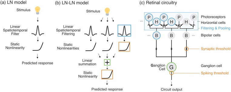
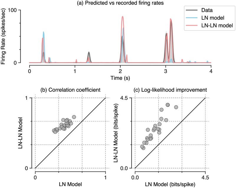
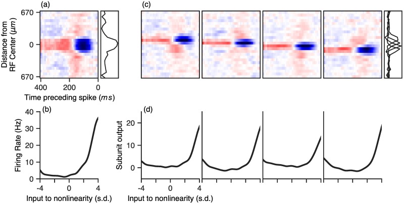
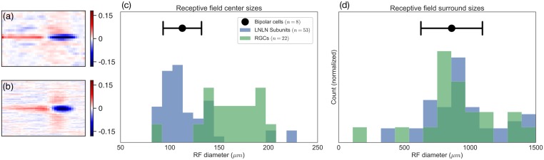
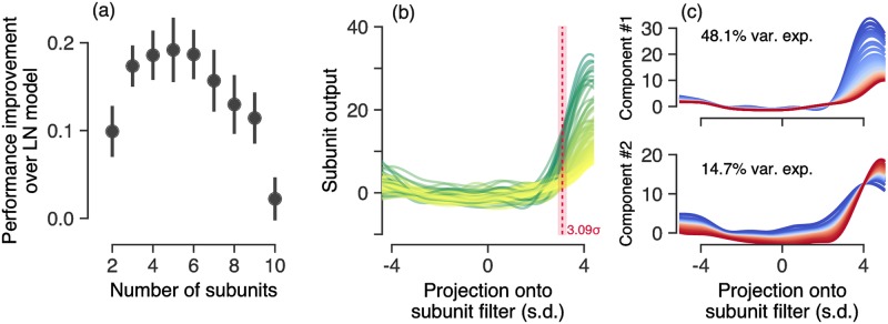
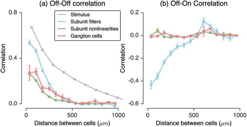
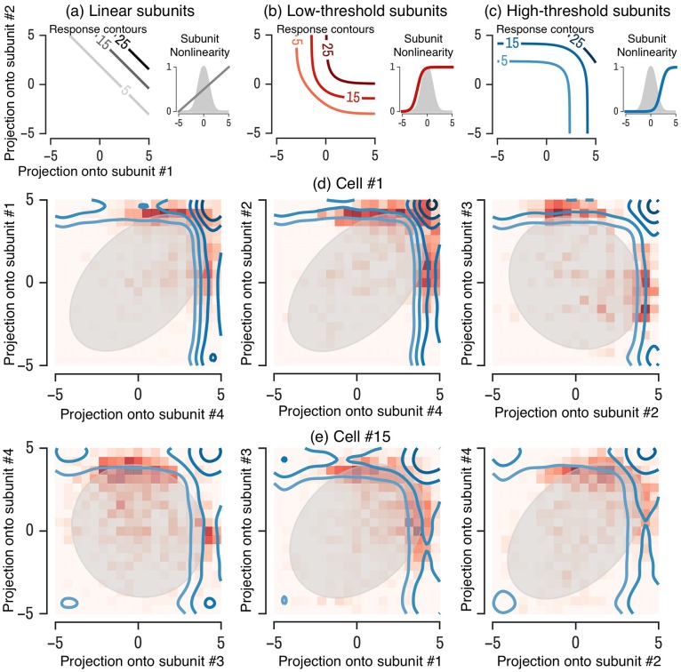
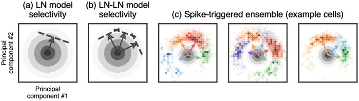
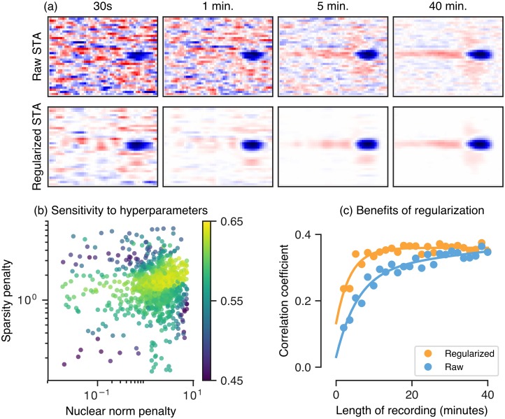
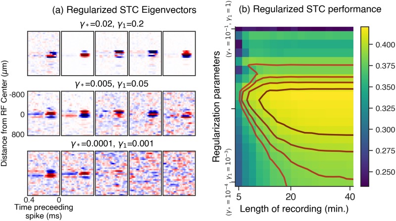
A central challenge in sensory neuroscience involves understanding how neural circuits shape computations across cascaded cell layers. Here we attempt to reconstruct the response properties of experimentally unobserved neurons in the interior of a multilayered neural circuit, using cascaded linear-nonlinear (LN-LN) models. We combine non-smooth regularization with proximal consensus algorithms to overcome difficulties in fitting such models that arise from the high dimensionality of their parameter space. We apply this framework to retinal ganglion cell processing, learning LN-LN models of retinal circuitry consisting of thousands of parameters, using 40 minutes of responses to white noise. Our models demonstrate a 53% improvement in predicting ganglion cell spikes over classical linear-nonlinear (LN) models. Internal nonlinear subunits of the model match properties of retinal bipolar cells in both receptive field structure and number. Subunits have consistently high thresholds, supressing all but a small fraction of inputs, leading to sparse activity patterns in which only one subunit drives ganglion cell spiking at any time. From the model's parameters, we predict that the removal of visual redundancies through stimulus decorrelation across space, a central tenet of efficient coding theory, originates primarily from bipolar cell synapses. Furthermore, the composite nonlinear computation performed by retinal circuitry corresponds to a boolean OR function applied to bipolar cell feature detectors. Our methods are statistically and computationally efficient, enabling us to rapidly learn hierarchical non-linear models as well as efficiently compute widely used descriptive statistics such as the spike triggered average (STA) and covariance (STC) for high dimensional stimuli. This general computational framework may aid in extracting principles of nonlinear hierarchical sensory processing across diverse modalities from limited data.


Conflict of interest statement

The authors have declared that no competing interests exist.

Figures

Fig 1
Fig 1. Schematic of the LN-LN model and corresponding retinal circuitry.
(a) The LN-LN cascade contains a bank of linear-nonlinear (LN) subunits, whose outputs are pooled at a second linear stage before being passed through a final nonlinearity. (b,c) The LN-LN model mapped on to a retinal circuit. The first LN stage consists of bipolar cell subunits and the bipolar-to-ganglion cell synaptic threshold. The second LN stage is pooling at the ganglion cell, plus a spiking threshold. The contribution of inhibitory amacrine cells is omitted here.
Fig 2
Fig 2. LN-LN models predict held-out response data better than LN models.
(a) Firing rates for an example neuron. The recorded firing rate (shaded, gray), is shown along with the LN model prediction (dashed, green) and the LN-LN prediction (solid, red). (b) LN-LN performance on held out data vs. the LN model, measured using correlation coefficient between the model and held out data. Note that all cells are above the diagonal. (c) Same as in (b), but with the performance metric of log-likelihood improvement over the mean rate in bits per spike.
Fig 3
Fig 3. Example LN-LN model parameters fit to a recording of an OFF retinal ganglion cell.
(a and b): LN-model parameters, consisting of a single spatial filter (a) and nonlinearity (b). (c and d) LN-LN model parameters. (c) First layer filters (top) and nonlinearities (bottom) of an LN-LN model fit to the same cell. Spatial profiles of filters are shown in gray to the right of the filters. The subunit filters have a much smaller spatial extent compared to the LN filter, but similar temporal profiles.
Fig 4
Fig 4. Comparison of subunit filter parameters with intracellular bipolar cell recordings.
(a) An example subunit bipolar cell. (b) A recorded bipolar cell receptive field. (c) Receptive field centers sizes for subunit filters (blue), LN model filters (green), and recorded bipolar cells (black point). (c) Same as in (b), but with receptive field surround sizes.
Fig 5
Fig 5. LN-LN model parameter analysis.
(a) Performance improvement (increase in correlation coefficient relative to an LN model) as a function of the number of subunits used in the LN-LN model. Error bars indicate the standard error across 23 cells. (b) Subunit nonlinearities learned across all ganglion cells. For reference the white noise input to a subunit nonlinearity has standard deviation 1, which sets the scale of the x-axis. Red line and shaded fill indicate the mean and s.e.m. of nonlinearity thresholds (see text for details). (c) Visualization of the principal axes of variation in subunit nonlinearities by adding or subtracting principal components from the mean nonlinearity. (top) The principal axis of variation in subunit nonlinearities results in a gain change, while (bottom) the second principal axis corresponds to a threshold shift. These two dimensions captured 63% of the nonlinearity variability across cells.
Fig 6
Fig 6. Decorrelation in LN-LN subunit models.
A naturalistic (pink noise) stimulus was shown to a population of nonlinear subunits. The correlation in the population after filtering at the subunit layer (blue), after the subunit nonlinearity (green), and after pooling and thresholding at the ganglion cell layer (red), in addition to the stimulus correlations (gray) are shown. Left: the correlation as a function of distance on the retina for Off-Off cell pairs. Right: correlation for Off-On cell pairs. For each plot, distances were binned every 70μm, and error bars are the s.e.m. within each bin.
Fig 7
Fig 7. Visualization of subunit contours.
Contours of equal firing probability are shown in a 2D space defined by the projection of the visual stimulus along each of two subunits. (a) Example contour plots for a model with low threshold subunit nonlinearities (inset) has concave contours. (b) A model with high threshold subunit nonlinearities has convex contours. (c & d) Contours from a model for two example ganglion cells, for three different pairs of subunits (left to right). In each panel, a histogram of the recorded firing rate is shown (red squares) as well as the stimulus distribution (gray oval).
Fig 8
Fig 8. Stimulus selectivity in LN and LN-LN models.
Each panel shows the raw stimulus distribution (gray contours) projected onto the top two principal components of the spike-triggered subunit activations (with subunits identified by the LN-LN model). The LN model (a) fires in response to stimuli in a single region, or cap, of stimulus space (indicated by the arrow and dashed threshold), whereas the LN-LN model (b) fires in response to a union of caps, each defined by an individual subunit. (c) Spike-triggered subunit activations for three representative cells are shown as colored histograms (colors indicate which model-identified subunit was maximally active during the spike), with the corresponding subunit filter directions shown as colored arrows (see text for details). Color intensity of the histogram indicates the probability density of the spike-triggered ensemble (STE), thus drops in intensity between changes in color indicate a multimodal STE, with high density modes centered near subunit filter directions.
Fig 9
Fig 9. Regularization for estimating receptive fields (via a regularized spike-triggered-average).
(a) Top row: the raw spike-triggered average computed using different amounts of data (from left to right, 30s to 40min), bottom row: the regularized spike-triggered average computed using the same amount of data as the corresponding column. (b) Performance (held-out log-likelihood) as a function of two regularization weights, the nuclear norm (x-axis, encourages low-rank structure) and the 1-norm (y-axis, encourages sparsity), for an example cell. (c) Correlation coefficient (on held-out data) between the firing rate of a retinal ganglion cell and LN model whose filter is fixed to be a regularized or raw (un-regularized) STA, as a function of the amount of training data for estimating the STA (length of recording).
Fig 10
Fig 10. Regularized spike-triggered covariance.
(a) Example panels of the output of our regularized spike-triggered covariance algorithm. Each panel contains the five most significant regularized eigenvectors of the STC matrix, reshaped as spatiotemporal filters. The bottom panel shows the result with no regularization added, and the upper panels show the result with increasing weights on the regularization penalties. Here γ1 is the regularization weight applied to an 1 penalty encouraging sparsity, and γ* is a regularization weight applied to a nuclear norm penalty, encouraging approximate spatiotemporal separability of the eigenvectors, when reshaped as spatiotemporal filters. (b) Summary across a population of cells. The heatmap shows the held-out performance of regularized STC (measured as the subspace overlap with the best fit LN-LN subspace, see text for details). The y-axis in (b) represents a line spanning 3 orders of magnitude in two-dimensional regularization parameter space (γ*, γ1), ranging from the point (γ* = 10−4, γ1 = 10−3) to (γ* = 10−1, γ1 = 1).

References

    1. Chichilnisky E. A simple white noise analysis of neuronal light responses. Network: Computation in Neural Systems. 2001;12(2):199–213. 10.1080/713663221 - DOI - PubMed
    1. Paninski L. Convergence properties of three spike-triggered analysis techniques. Network: Comput Neural Syst. 2003;14:437–464. 10.1088/0954-898X/14/3/304 - DOI - PubMed
    1. Schwartz O, Pillow JW, Rust NC, Simoncelli EP. Spike-triggered neural characterization. Journal of Vision. 2006;6(4). 10.1167/6.4.13 - DOI - PubMed
    1. Aljadeff J, Lansdell BJ, Fairhall AL, Kleinfeld D. Analysis of neuronal spike trains, deconstructed. Neuron. 2016;91(2):221–259. 10.1016/j.neuron.2016.05.039 - DOI - PMC - PubMed
    1. Van Steveninck RDR, Bialek W. Real-time performance of a movement-sensitive neuron in the blowfly visual system: coding and information transfer in short spike sequences. Proceedings of the Royal Society of London B: Biological Sciences. 1988;234(1277):379–414. 10.1098/rspb.1988.0055 - DOI

Publication types

LinkOut - more resources