Calcium imaging and dynamic causal modelling reveal brain-wide changes in effective connectivity and synaptic dynamics during epileptic seizures

Abstract

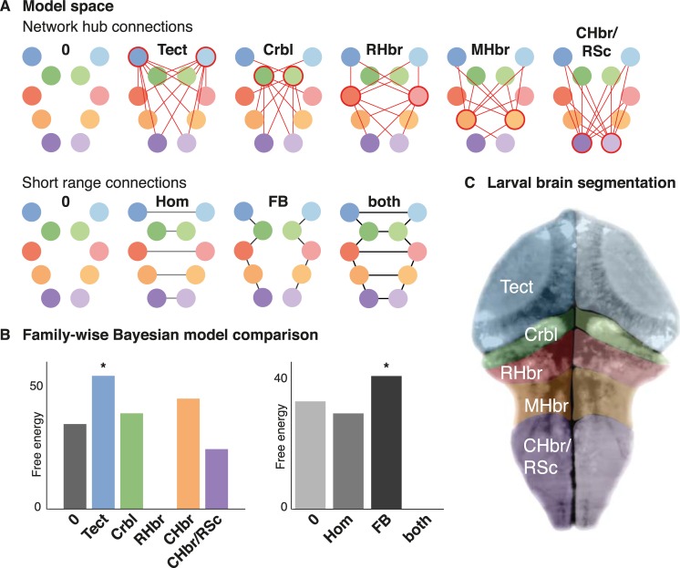
Pathophysiological explanations of epilepsy typically focus on either the micro/mesoscale (e.g. excitation-inhibition imbalance), or on the macroscale (e.g. network architecture). Linking abnormalities across spatial scales remains difficult, partly because of technical limitations in measuring neuronal signatures concurrently at the scales involved. Here we use light sheet imaging of the larval zebrafish brain during acute epileptic seizure induced with pentylenetetrazole. Spectral changes of spontaneous neuronal activity during the seizure are then modelled using neural mass models, allowing Bayesian inference on changes in effective network connectivity and their underlying synaptic dynamics. This dynamic causal modelling of seizures in the zebrafish brain reveals concurrent changes in synaptic coupling at macro- and mesoscale. Fluctuations of both synaptic connection strength and their temporal dynamics are required to explain observed seizure patterns. These findings highlight distinct changes in local (intrinsic) and long-range (extrinsic) synaptic transmission dynamics as a possible seizure pathomechanism and illustrate how our Bayesian model inversion approach can be used to link existing neural mass models of seizure activity and novel experimental methods.

Fig 1. Dynamic causal modelling results of simulated calcium imaging time traces.

(A) Left hand side time series show signal amplitude over time in arbitrary units. Calcium imaging dynamics were modelled by convolving LFP-traces (top) with a calcium imaging kernel (middle), resulting in a CAI time trace (bottom). The CAI trace follows slow LFP dynamics, whilst attenuating faster components of the original signal. Right hand side frequency plots show normalised log-amplitude derived from a Fourier transform of respective time series over a range of frequencies (1-50Hz). In frequency space, the convolution differentially scales low and high frequency components, but preserves most frequency features. (B) LFP-like time series plotted in arbitrary amplitude units over 10s. These are derived from a three-population neural mass model with increasing values of a single parameter, H₁—also shown in Fig 1C. Example CAI traces after convolution are shown in darker colours. (C) A three-population neural mass model is used for generating LFP traces, and is subsequently fitted to the convolution-derived CAI traces. (D) Bayesian model comparison (Bayes factor 2.6) between repeated model inversions identifies correctly that differences between simulated CAI traces were caused by the effects of variations in the H₁ parameter on the synthetic LFP traces. The parameter values included in the generative model are shown in the bar chart. (E) The DCM analysis provides estimates of the generative model parameters (shown in the bar chart). These results correctly infer the increase of H₁ across the six model inversions from the CAI traces. Parameter estimates are shown here with a Bayesian 95% confidence interval (grey bars). Whilst the group mean parameter value and the effect size are different, this inversion correctly identifies the linear increase in the parameter from the simulated CAI dataset. LFP–local field potential, CAI–calcium imaging, DCM–dynamic causal model, PEB–parametric empirical Bayes.

Fig 2. PTZ-iduced seizures recorded in the zebrafish larvae using light sheet imaging.

(A) This image shows heat maps of fluorescence in a single slice of the intact larval zebrafish brain in the xy plane at different time points during the experiment (time points also indicated in Fig 2B). Seizure activity (t₂) is visually apparent as an overall increase in neuronal activity compared to baseline state (t₁). (B) Regionally averaged time traces of the fluorescence signal across 5 bilateral anatomically defined regions are shown for the whole duration of the experiment in a single animal (150 minutes). Seizures are readily apparent as an inrease in generalised and apparently synchronous high amplitude activity. (C) Average Fourier power spectra across fish and across all brain regions are plotted against time for the duration of the experiment, using a sliding window estimator (length: 60s, step: 10s), with colours indicating log-power. The graph is a the average over n = 3 fish. PTZ causes an increase largely in low frequencies (<2Hz), with intermittent bursts of more broadband activity. (D) A correlation matrix showing correlation indices of the power-distribution patterns across different time points (delay-delay matrix). This reveals three distinct time periods, corresponding to baseline (<30min), ictal (30-70min) and late ictal (>70min) phases with distinct spectral signatures and temporal dynamics. Tect—Tectum, Crbl—Cerebellum, RHbr—Rostral Hindbrain, MHbr—Mid-Hindbrain, CHbr/RSc—Caudal Hindbrain/Rostral Spinal Cord.

Fig 3. Network model architecture during interictal background activity.

(A) Two aspects of a factorial model space are shown: extrinsic connectivity of putative network hubs (yielding 6 types of models), and short range connection between neighbouring and homotopic nodes (yielding 4 different types of models); a total of 6 * 4 = 24 models were evaluated, where any one model is combines one of the network hub connectivity architectures with a short-range connectivity setup. Bayesian model reduction was used to estimate the model evidence across this model space characterised by the presence or absence of these defined sets of between-region reciprocal connections (neighbouring, homotopic, and hub connections). (B) For each model family (corresponding to the factorial model space), the free energy difference to the worst-performing model is shown. In DCM, the free energy difference is used to approximate model log-likelihood differences: Asterisks indicate the winning model family identified from Bayesian model selection. These results indicate that the model with neighbouring, and homotopic connections as well as the optic tectum with hub-like connectivity best explain the observed spontaneous activity at baseline. (C) Mapping of the ROIs for this analysis is illustrated as overlay on a single fluorescence image taken from one of the animals included in this study. Areas were identified based on visible neuroanatomical landmarks and correspond to the nodes of the same colour in the network representations of the model space.

Fig 4. Group level effects of PTZ-induced seizures on synaptic coupling.

(A) Here (1) an example fluorescence time trace from a single region, (2) an example eigenmode summary of the cross-spectral density changes over time observed across all region in a single fish (this is derived from a multivariate autoregressive model and constitutes the primary data features in DCM), and (3) the model fits of windowed DCMs to that same animal are shown. The middle and bottom panel both plot frequency power distribution across the time of the experiment, where the log-power for any given frequency is represented by colours corresponding to the same colourbar (range -4 to 2). DCMs fitted to these individual time windows capture the spectral changes measured well for the duration of the experiment. (B) Free energy approximation for the model-family evidence for reduced models where PTZ-induced changes were restricted to a subset of coupling parameters is shown. Bayesian model comparison at this second (between time-window) level was performed to compare reduced models with PTZ-induced changes in F forward, B backward, FB both, 0 or neither type of regional connectivity. Asterisks indicate the winning models. Only changes in connections from other brain regions to the hub region show evidence of being modulated by the seizure activity. (C) Similarly, free energies for model families that allow for intrinsic connectivity parameter changes in none of the brain regions, single brain regions, or all brain regions are shown. The asterisk indicates the winning model. There was strong evidence for intrinsic connection changes in all brain regions. (D) Estimates of the PTZ-effect on DCM model parameters are shown, corresponding to the expected change relative to baseline that was induced by PTZ. Each dot represents a posterior density, centred around the expected value, and its size inversely correlated to the covariance (or uncertainty), i.e. the larger the dot, the more precise the estimate. Dots are colour-coded by region as shown in the legend. Lines indicate the median of the expected values with whiskers showing 25^th and 75^th centiles respectively–but note that individual parameter estimates are not random samples from an underlying distribution but themselves represent more or less precise model parameters fitted to the observed data. Model families (extrinsic): 0 –no extrinsic connectivity changes; F–extrinsic connectivity changes in forward connections only; B–extrinsic connectivity changes in backward connections only; FB–extrinsic connectivity changes in both forward and backward connections. Model families (intrinsic): 0 –no intrinsic connectivity changes; Tect–intrinsic connectivity changes only in the bilateral optic tectum; Crbl–intrinsic connectivity changes only in the bilateral cerebellum; RHbr–intrinsic connectivity changes only in the rostral hindbrain; MHbr–intrinsic connectivity changes only in the mid-hindbrain; CHbr/RSc–intrinsic connectivity changes only in the caudal hindbrain/rostral spinal cord; all–intrinsic connectivity changes across all areas.

Fig 5. Temporal evolution of intrinsic coupling parameter changes in the optic tectum throughout the seizure.

(A) A single source 3-population model is shown, indicating the seven parameters that are fitted as part of the dynamic causal modelling: 5 intrinsic connectivity parameters (H₁ –H₃ excitatory connections, to H₄ –H₅ inhibitory connections), and 2 time constants (T_I and T_E). (B) A principal component analysis was performed separately across the posterior estimates of intrinsic connectivity, and time-constant parameters for the optic tectum across all time windows of the experiment. The coefficients for the first principal component of intrinsic connections (left) and time constants (right) are shown here. (C) Using these two principal components, parameter estimates of intrinsic coupling within the optic tectum for each individual time window are projected onto a two-dimensional parameter space. Each point of this projection is colour coded according to its time in the experiment from which the estimate was derived. In order to relate location in parameter space to spectral output at the optic tectum, for each point in this parameter space, we ran a dynamic causal model of the optic tectum in simulation mode to yield an yield an estimate of power spectral densities at that particular parameter combination. Here we map the predicted mean log-power in the delta- (black and white heat map) and gamma-band (purple isoclines) respectively. Thus the figure shows the temporal evolution of intrinsic coupling parameter estimates within the optic tectum during the seizures on a map of the spectral energy for different frequency bands for the specific parameter combinations. Time points just after PTZ injection occupy the most extreme top-right corner of this parameter space. This indicates both slower inhibitory connectivity (time constant component) and stronger excitatory / weaker inhibitory connectivity (connectivity time constant component). These paramete changes are associated with high powers in both the gamma and the delta band.

References

1. Thomas RH, Berkovic SF. The hidden genetics of epilepsy—a clinically important new paradigm. Nat Rev Neurol. 2014; 10(5):283–92. 10.1038/nrneurol.2014.62 - DOI - PubMed
1. Parker L, Padilla M, Du Y, Dong K, Tanouye M a. Drosophila as a model for epilepsy: bss is a gain-of-function mutation in the para sodium channel gene that leads to seizures. Genetics. 2011; 187(2):523–34. 10.1534/genetics.110.123299 - DOI - PMC - PubMed
1. Depaulis A, David O, Charpier S. The genetic absence epilepsy rat from Strasbourg as a model to decipher the neuronal and network mechanisms of generalized idiopathic epilepsies. J Neurosci Methods. 2015;:1–16. - PubMed
1. Seo S, Leitch B. Altered thalamic GABAA-receptor subunit expression in the stargazer mouse model of absence epilepsy. Epilepsia. 2014; 55(2):224–32. 10.1111/epi.12500 - DOI - PubMed
1. Dhindsa RS, Goldstein DB. Genetic Discoveries Drive Molecular Analyses and Targeted Therapeutic Options in the Epilepsies. Curr Neurol Neurosci Rep. 2015; 15(10):70 10.1007/s11910-015-0587-4 - DOI - PubMed
Publication types
LinkOut - more resources