Analysis of Epistasis in Natural Traits Using Model Organisms

Abstract

The ability to detect and understand epistasis in natural populations is important for understanding how biological traits are influenced by genetic variation. However, identification and characterization of epistasis in natural populations remains difficult due to statistical issues that arise as a result of multiple comparisons, and the fact that most genetic variants segregate at low allele frequencies. In this review, we discuss how model organisms may be used to manipulate genotypic combinations to power the detection of epistasis as well as test interactions between specific genes. Findings from a number of species indicate that statistical epistasis is pervasive between natural genetic variants. However, the properties of experimental systems that enable analysis of epistasis also constrain extrapolation of these results back into natural populations.

Keywords: allele frequency; epistasis; mechanism of epistasis; natural genetic variation.

Figure 1:. Primer on measuring pairwise epistasis in a natural population.

There are three primary steps to measuring statistical epistasis in a pairwise manner. Here, we illustrate its detection in a haploid population (e.g. S. cerevisiae) between two loci (A and B) containing two alleles. We have chosen this example to demonstrate how allele frequencies can impact estimates of statistical epistasis and the additive terms of the model. Reading Box 2 in concert with this figure should be helpful. A. To estimate epistasis, a number of individuals must be sampled from a larger population. Here we show how three subpopulations can be sampled from a larger population of genotypically unique individuals (illustrated by different colors). These populations might be geographical in nature (i.e. yeast from the US vs yeast from China). B. The sampled individuals are then genotyped and phenotyped to create a data matrix (N = 200 for each population). For a haploid, there are four possible genotypes between two allele pairs. Only one data matrix is displayed, but each population is assumed to have its own data matrix. The allele frequency at A and B can be calculated for each population using the Geno column. The phenotypic variance can be calculated for each population using the Pheno column. In this case, the allele frequencies for both loci are different in the three populations. C. The data from B are fit using linear regression. In these plots, the genotypes of both loci are represented by the x-axis (A) or color of the points. Non-additivity can be recognized by non-parallelism between the blue and yellow lines; the three populations differ in allele frequency across loci. To simulate how allele frequency affects the distribution of phenotypes in a population, first we assumed an epistatic relationship between the loci, as represented in the top row. This relationship does not vary across populations because we assumed no higher-order epistasis existed. Next, random noise (from a Gaussian distribution) was added to the individual phenotypes, to represent variation contributed by the environment, stochasticity, or other loci (the average of which is constant across populations). Each individual’s phenotype is represented by a single dot in the middle and bottom rows. The regression lines between the middle and bottom rows differ according to the regression model; in the middle, the additive model given by Equation (2) in Box 2 was used, in the bottom, the non-additive model that includes statistical epistasis, given by Equation (1) in Box 2, was used. The amount of variance that is captured by the fit is also shown on each panel. V_G, V_A, and V_I are defined in Box 2. As can be seen, for two allele pairs with high levels of epistasis, allele frequency plays an important role in the slope of the fit (i.e. the direction of the effect size) and the amount of variance captured by the strictly additive model (middle row).

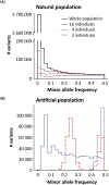
Figure 2:. Allele frequencies in natural and artificial populations.

A. Histogram of allele frequencies of genetic variants in a human population (black line). These data were taken from 2,504 sequenced individuals as part of the 1000 Genomes project, limiting data to chromosome I. The population allele frequencies of genetic variants that differ between two, four, or sixteen individuals is also plotted, showing that while most genetic variation in a population is rare, most genetic variation between two individuals is common. B. Histogram of allele frequencies of genetic variants in an artificial mapping population constructed from either two, four, or sixteen parental lines (colors and line types follow A). The amount of genetic variation captured in the parents and initial allele frequencies are taken from data in A. While the exact allele frequency histograms will vary between species due to idiosyncratic differences, these panels illustrate the inflation of allele frequencies that will occur due to construction of an artificial population.

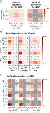
Figure 3:. Genotype frequencies in natural and artificial populations.

The genotype frequencies of a natural or artificial (inbred) diploid population (N = 10000 or 256 respectively), shown as a heatmap. The artificial population was created from either a 2, 4, or 16 parent standard RIL cross design. The different population sizes (N) match typical sizes used with natural or artificial populations. There are nine possible genotypes for two allele pairs in a diploid, here represented as colored cells within each 3×3 matrix, which vary in the allele frequencies of either A or B (given by p_A1 and p_B2). The genotype of locus A is shown on the y-axis and the genotype of locus B is shown on the x-axis. For rare genotypes (<100 in A and < 10 in B), the exact number of expected individuals is also shown. If sufficient rounds of inbreeding occur, genotypes for artificial populations will be homozygous. For clarity, the impossible heterozygous genotypes are shown in grey for artificial populations. A. Comparison of genotype frequencies for natural and artificial populations. The allele frequency of each allele is 50%. For natural populations, individuals were assumed to follow Hardy-Weinberg equilibrium, and the most-likely genotype is the double heterozygote. For artificial populations, each of the four possible homozygote combinations are equally likely. B. Comparison of genotype frequencies in natural populations for three different allele frequencies. The case of p = 0.5% represents rare variants, p = 5% represents common variants, and p = 50% represents allele frequencies where detection of epistasis is maximally powered (Max). Rare variants do not explore much of the genotype space (i.e. rare-rare only one genotype is > 100, rare-common only two genotypes are > 100 and rare-max only three genotypes are > 100). C. For artificial populations, individuals were assumed to be completely inbred, resulting in only four possible genotypes (the corners of the square). The case of p = 6.25% represents allele frequencies that are possible in a 16 parent RIL, p = 25% represents allele frequencies that are possible in a 4 or 16 parent RIL, and p = 50% represents allele frequencies that are possible in a 2, 4 or 16 parent RIL.

References

1. Cutting GR (2010) Modifier genes in Mendelian disorders: the example of cystic fibrosis. Ann N Y Acad Sci 1214, 57–69. - PMC - PubMed
1. Marouli E et al. (2017) Rare and low-frequency coding variants alter human adult height. Nature 542 (7640), 186–190. - PMC - PubMed
1. Visscher PM et al. (2012) Five years of GWAS discovery. Am J Hum Genet 90 (1), 7–24. - PMC - PubMed
1. Cordell HJ (2002) Epistasis: what it means, what it doesn't mean, and statistical methods to detect it in humans. Hum Mol Genet 11 (20), 2463–8. - PubMed
1. Phillips PC (2008) Epistasis--the essential role of gene interactions in the structure and evolution of genetic systems. Nat Rev Genet 9 (11), 855–67. - PMC - PubMed
LinkOut - more resources