. 2018 Nov;210(3):809-819.
doi: 10.1534/genetics.118.301298. Epub 2018 Aug 31.

Can Deep Learning Improve Genomic Prediction of Complex Human Traits?

Affiliations

Can Deep Learning Improve Genomic Prediction of Complex Human Traits?

Pau Bellot et al. Genetics. 2018 Nov.

Abstract

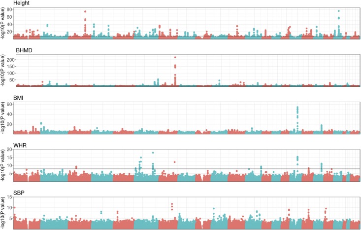
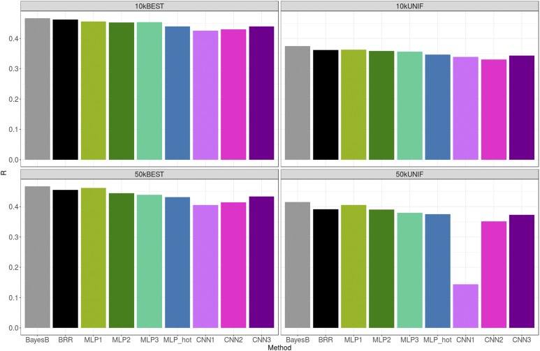
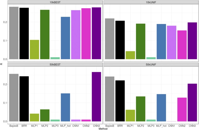
The genetic analysis of complex traits does not escape the current excitement around artificial intelligence, including a renewed interest in "deep learning" (DL) techniques such as Multilayer Perceptrons (MLPs) and Convolutional Neural Networks (CNNs). However, the performance of DL for genomic prediction of complex human traits has not been comprehensively tested. To provide an evaluation of MLPs and CNNs, we used data from distantly related white Caucasian individuals (n ∼100k individuals, m ∼500k SNPs, and k = 1000) of the interim release of the UK Biobank. We analyzed a total of five phenotypes: height, bone heel mineral density, body mass index, systolic blood pressure, and waist-hip ratio, with genomic heritabilities ranging from ∼0.20 to 0.70. After hyperparameter optimization using a genetic algorithm, we considered several configurations, from shallow to deep learners, and compared the predictive performance of MLPs and CNNs with that of Bayesian linear regressions across sets of SNPs (from 10k to 50k) that were preselected using single-marker regression analyses. For height, a highly heritable phenotype, all methods performed similarly, although CNNs were slightly but consistently worse. For the rest of the phenotypes, the performance of some CNNs was comparable or slightly better than linear methods. Performance of MLPs was highly dependent on SNP set and phenotype. In all, over the range of traits evaluated in this study, CNN performance was competitive to linear models, but we did not find any case where DL outperformed the linear model by a sizable margin. We suggest that more research is needed to adapt CNN methodology, originally motivated by image analysis, to genetic-based problems in order for CNNs to be competitive with linear models.

Keywords: Convolutional Neural Networks; GenPred; Genomic Prediction regressions; Multilayer Perceptrons; UK Biobank; complex traits; deep learning; genomic prediction; whole-genome.


Figures

Figure 1
Figure 1
Representation of a Multilayer Perceptron. Each layer is connected to the previous one by a weighted linear summation, here represented by weight matrices W(i), and a (non)linear transformation. Redrawn from http://www.texample.net/tikz/examples/neural-network/.
Figure 2
Figure 2
Representation of a Convolutional Neural Network. (a) The input layer consists of the SNP matrix. The convolution filters are the same through all different SNPs; we slide these filters horizontally with a stride of “s” SNPs, i.e., the number of SNPs that the filter is moved to compute the next output. (b) Neuron outputs of convolutional layer with K dimensions (outlined as blue and green squares) are computed from inputs of input layer, which fall within their receptive field (here consecutive sets of three SNPs) in the layer below (shown as blue- and green-colored rectangles). (c) Convolutional networks usually include pooling layers, combining the output of the previous layer at certain locations into a single neuron (here, a 1 × 2 pooling is outlined in yellow). (d) Fully connected layers connect every neuron in one layer to every neuron in another layer. It is the same as traditional MLPs, finally obtaining an estimated output (e). Partly redrawn using code in http://www.texample.net/tikz/examples/neural-network/.
Figure 3
Figure 3
Genome-wide association study of traits analyzed. Each dot represents the P-value (−log10 scale) of a single SNP. SNPs from different chromosomes are represented by alternating colors, starting with chromosome 1 on the left. The horizontal line indicates the tentative genome-wide significance level (P-value = 10−8). BHMD, bone heel mineral density; BMI, body mass index; SBP, systolic blood pressure; WHR, waist–hip ratio.
Figure 4
Figure 4
Prediction performance across methods and SNP sets for height. Gray, green, blue, and magenta bars correspond to linear, MLP, one-hot encoding MLP, and CNN methods, respectively. Average SE of R’s were ∼3 × 10⁻³. BEST, set with the 10k or 50k top most-associated SNPs; BRR, Bayesian Ridge Regression; CNN, Convolutional Neural Network; MLP, Multilayer Perceptron; UNIF, set in which the genome was split in windows of equal physical length and the most-associated SNP within each window was chosen.
Figure 5
Figure 5
Prediction performance across methods and SNP sets for bone heel mineral density. Gray, green, blue, and magenta bars correspond to linear, MLP, one-hot encoding MLP, and CNN methods, respectively. Very low bar means method not converging. Average SE of R’s were ∼3 × 10⁻³. BEST, set with the 10k or 50k top most-associated SNPs; BRR, Bayesian Ridge Regression; CNN, Convolutional Neural Network; MLP, Multilayer Perceptron; UNIF, set in which the genome was split in windows of equal physical length and the most-associated SNP within each window was chosen.
Figure 6
Figure 6
Histogram of distances and correlations between consecutive SNPs in the 10k BEST (the 10k top most-associated SNPs) and UNIF (the genome was split in windows of equal physical length and the most-associated SNP within each window was chosen) sets. (a) Distances (dist) in base pairs (log10 units) between consecutive SNPs, within the same chromosome. (b) Absolute value of correlation [abs(corr)] between genotype values of consecutive SNPs when each genotype is coded as 0, 1, or 2.

References

    1. Abadi M., Agarwal A., Barham P., Brevdo E., Chen Z., et al. , 2015. TensorFlow: large-scale machine learning on heterogeneous systems. Available at: tensorflow.org. Accessed: July 1, 2018.
    1. Alipanahi B., Delong A., Weirauch M. T., Frey B. J., 2015. Predicting the sequence specificities of DNA- and RNA-binding proteins by deep learning. Nat. Biotechnol. 33: 831–838. 10.1038/nbt.3300 - DOI - PubMed
    1. Chang C. C., Chow C. C., Tellier L. C., Vattikuti S., Purcell S. M., et al. , 2015. Second-generation PLINK: rising to the challenge of larger and richer datasets. Gigascience 4: 7 10.1186/s13742-015-0047-8 - DOI - PMC - PubMed
    1. Chollet F., 2015. Keras: deep learning library for theano and tensorflow. Available at: https://keras.io/. Accessed May 1, 2018.
    1. de Los Campos, G., and A. Grueneberg, 2017 BGData: a suite of packages for analysis of big genomic data. R package version 1.0.0.9000. Available at:https://github.com/QuantGen/BGData - PMC - PubMed

Publication types

LinkOut - more resources