Attractor-like Dynamics in Belief Updating in Schizophrenia

Abstract

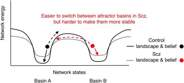
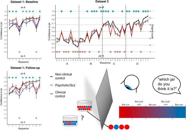
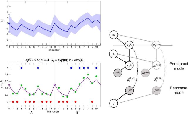
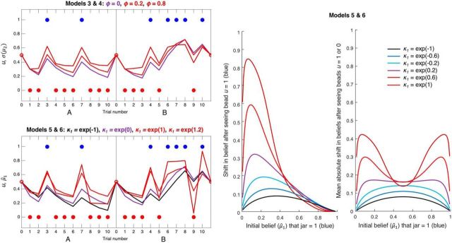
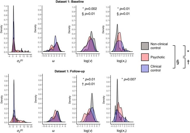
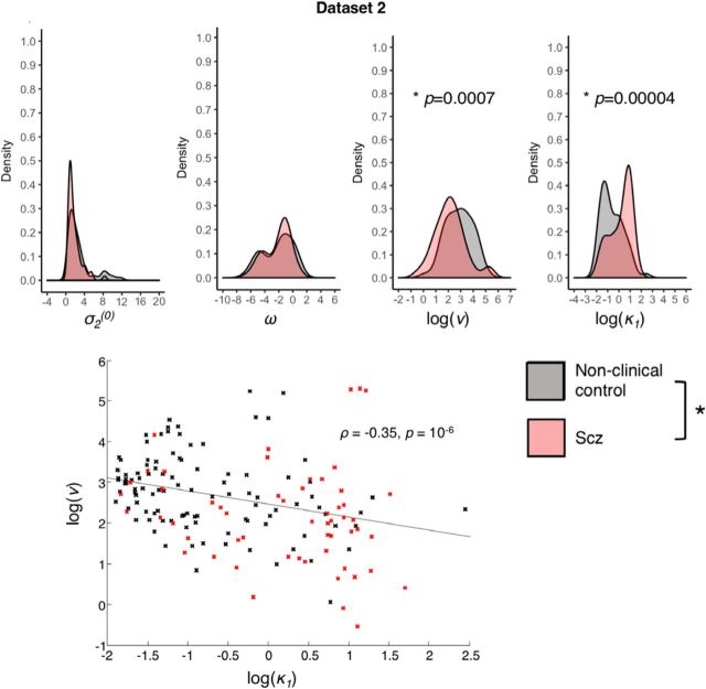
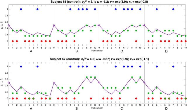
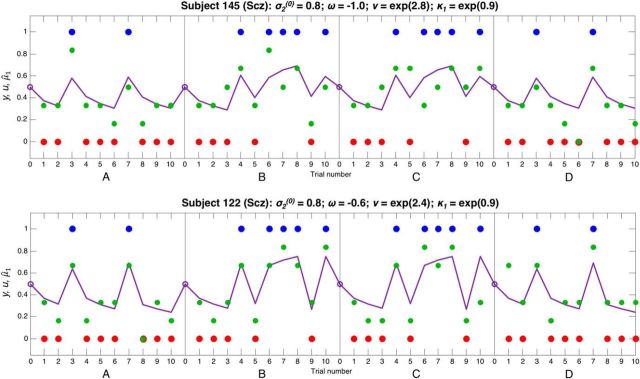
Subjects with a diagnosis of schizophrenia (Scz) overweight unexpected evidence in probabilistic inference: such evidence becomes "aberrantly salient." A neurobiological explanation for this effect is that diminished synaptic gain (e.g., hypofunction of cortical NMDARs) in Scz destabilizes quasi-stable neuronal network states (or "attractors"). This attractor instability account predicts that (1) Scz would overweight unexpected evidence but underweight consistent evidence, (2) belief updating would be more vulnerable to stochastic fluctuations in neural activity, and (3) these effects would correlate. Hierarchical Bayesian belief updating models were tested in two independent datasets (n = 80 male and n = 167 female) comprising human subjects with Scz, and both clinical and nonclinical controls (some tested when unwell and on recovery) performing the "probability estimates" version of the beads task (a probabilistic inference task). Models with a standard learning rate, or including a parameter increasing updating to "disconfirmatory evidence," or a parameter encoding belief instability were formally compared. The "belief instability" model (based on the principles of attractor dynamics) had most evidence in all groups in both datasets. Two of four parameters differed between Scz and nonclinical controls in each dataset: belief instability and response stochasticity. These parameters correlated in both datasets. Furthermore, the clinical controls showed similar parameter distributions to Scz when unwell, but were no different from controls once recovered. These findings are consistent with the hypothesis that attractor network instability contributes to belief updating abnormalities in Scz, and suggest that similar changes may exist during acute illness in other psychiatric conditions.SIGNIFICANCE STATEMENT Subjects with a diagnosis of schizophrenia (Scz) make large adjustments to their beliefs following unexpected evidence, but also smaller adjustments than controls following consistent evidence. This has previously been construed as a bias toward "disconfirmatory" information, but a more mechanistic explanation may be that in Scz, neural firing patterns ("attractor states") are less stable and hence easily altered in response to both new evidence and stochastic neural firing. We model belief updating in Scz and controls in two independent datasets using a hierarchical Bayesian model, and show that all subjects are best fit by a model containing a belief instability parameter. Both this and a response stochasticity parameter are consistently altered in Scz, as the unstable attractor hypothesis predicts.

Keywords: Bayesian; attractor model; beads task; disconfirmatory bias; psychosis; schizophrenia.

Figure 1.

Effects of attractor network dynamics on belief updating. This schematic illustrates the energy landscapes of two Hopfield-type networks each with two basins of attraction. Continuous black line indicates a normal network whose basins of attraction are relatively deep. Dotted black line indicates the effect of NMDAR (or cortical dopamine 1 receptor) (Durstewitz and Seamans, 2008; Redish et al., 2007) hypofunction (Abi-Saab et al., 1998; Javitt et al., 2012) on the energy landscape: the attractor basins become more shallow. We assume that Basins A and B correspond to different inferences about (hidden) states in the world (e.g., one jar or another being the source of beads in the beads task). Dots indicate the networks' representations of either control or Scz subjects' beliefs about these hidden states. Such networks are highly reminiscent of Hopfield networks with two stored representations; in this case, the representations correspond to inferences about hidden states, rather than memories. Arrows indicate the changes in network states resulting from sensory evidence for (solid arrows) or against (dashed arrows) the current inference. When the attractor basin is shallower, it is harder for supportive evidence to stabilize the current state much further, but it is easier for contradictory evidence, or just stochastic neuronal firing, to shift the current network state toward an alternative state. These changes in network dynamics may also be reflected in the inferences the network computes (i.e., easier switching between attractor basins may correspond to easier switching between beliefs), although this is yet to be demonstrated experimentally. NMDAR hypofunction could contribute to an increased tendency to switch between beliefs and increased stochasticity in responding in several ways (Rolls et al., 2008): (1) by reducing inhibitory interneuron activity, via weakened NMDAR synapses from pyramidal cells to interneurons, such that other attractor states are less suppressed when one is active (a spiking network model has shown that this leads to more rapid initial belief updating in perceptual tasks) (Lam et al., 2017); (2) by reducing pyramidal cell activity, via weakened recurrent NMDAR synapses on pyramidal cells, such that attractor states are harder to sustain; and (3) by reducing the NMDAR time constant, making states more vulnerable to random fluctuations in neural activity. See also similar schematics elsewhere (Durstewitz and Seamans, 2008; Rolls et al., 2008).

Figure 2.

Beads task schematic and group average confidence ratings in Datasets 1 and 2. Bottom right, Schematic of the beads task: two jars containing opposite proportions of beads are concealed from view, and a subject is asked to rate the probability of either jar being the source of a sequence of beads he/she is viewing (after each bead in turn). Top left, Mean (± SE) confidence ratings in the blue jar over the 10-bead sequence averaged across each group at baseline in Dataset 1. Bottom left, Same quantities at follow-up in Dataset 1. Top right, Quantities in four 10-bead sequences concatenated together (they were presented to the subjects separately during testing) in Dataset 2.

Figure 3.

The structure of the HGF (Model 6) and some simulated data. Top left, The evolution of μ₂, the posterior estimate of tendency x₂ toward the blue (positive) or red (negative) jar, is plotted over two concatenated series of 10 trials (the first two in Dataset 2). The estimate of the tendency on trial k + 1, μ₂^(k+1), is selected from a Gaussian distribution with mean μ₂^(k) (blue line) and variance σ₂^(k) + exp(ω) (blue shading). ω is a static source of variance at this level. The initial variance σ₂⁽⁰⁾ (along with ω) affects the size of initial updates, so we estimated this parameter (which is often fixed). Bottom left, The beads seen by the subjects, u^(k) (blue and red dots) and the response model. The response model maps from μ̂₁^(k+1) (purple line), the prediction of x₁ on the next trial, which is a sigmoid function s of μ₂^(k) (or of (κ₁μ₂^(k)) in Models 5 and 6), to y^(k), the subject's indicated estimate of the probability the jar is blue (green dots). Variation in this mapping is modeled as the precision ν of a β distribution. Right, Schematic representation of the generative model in Models 5 and 6 (i.e., including κ₁). Black arrows indicate the probabilistic network on trial k. Gray arrows indicate the network at other points in time. The perceptual model lies above the dotted arrows, and the response model below them. Shaded circles represent known quantities. Unshaded circles represent estimated parameters and states. Dotted line indicates the result of an inferential process (the response model builds on a perceptual model inference). Solid lines indicate generative processes.

Figure 4.

Simulated data illustrating the effects of ϕ (Models 3 and 4) and κ₁ (Models 5 and 6) on inference. Both panels represent simulated perceptual model predictions in the same format as before, with σ₂⁽⁰⁾ and ω set to their previous values; hence, the purple line in these plots is identical to that in Figure 3. The second level and simulated responses y have been omitted for clarity. Top left, Simulations of a perceptual model incorporating an autoregressive order (1) process at the second level, using three different values of AR(1) parameter ϕ: 0, 0.2, and 0.8. The estimate of the tendency on trial k + 1, μ₂^(k+1), is selected from a Gaussian distribution with mean μ₂^(k) + ϕ(m − μ₂^(k)) and variance σ₂^(k) + exp(ω). Over time, μ₂ is therefore attracted toward level m (fixed to 0, i.e., at σ(μ₂) = 0.5) at a rate determined by ϕ. In effect, this gives the model a 'disconfirmatory bias,' such that as ϕ increases, σ(μ₂) is pulled further away from a belief in either jar, and toward 0.5 (maximum uncertainty about the jars). Bottom left, Simulations of a perceptual model using four different values of scaling factor κ₁, which alters the sigmoid transformation: μ̂₁^(k+1) = s(κ₁ · μ₂^(k)). When κ₁ > exp(0), updating is greater to unexpected evidence and lower to consistent evidence; when κ₁ < exp(0), the reverse is true. Red and brown lines (κ₁ > exp(0)) indicate the effects of increasingly unstable attractor networks; that is, switching between states (jars) becomes more likely (a concomitant increase in vulnerability to noise, i.e., response stochasticity, is not shown). Green line (κ₁ = exp(−1)) indicates slower updating around μ̂₁ = 0.5, as was found in controls. κ₁ permits a greater range of updating patterns than ϕ (the green and brown trajectories in the bottom cannot be produced by Model 4), which may be why Model 6 can fit both controls and Scz groups well. Middle, Plot represents the effects of κ₁ on belief updating, as a function of the initial belief μ̂₁ (σ₂⁽⁰⁾ and ω were set to 1.5 and −1, respectively, as in Fig. 5; changing these parameters does not qualitatively alter the effects of κ₁ shown here). For values of κ₁ < exp(0) = 1 (bottom three curves) and initial beliefs to the left of these curves' maxima (i.e., that the jar is probably red), relatively small increases in μ̂₁ are made if one blue bead (u = 1) is observed, such that the subject still believes the jar is most likely red. For values of κ₁ > exp(0.5) (top two curves), observing one blue bead causes such a large update for all but the most certain initial beliefs in a red jar that the subject's posterior belief is that the jar is probably blue. These subjects' beliefs are no longer stable, but neither can they reach certainty: only tiny updates toward 1 are possible for μ̂₁ > 0.8. Right, Plot represents the average absolute shifts in beliefs on observing beads of either color. This 'vulnerability to updating' is highly reminiscent of the 'energy state' of a neural network model (schematically illustrated in Fig. 1) (i.e., in low energy states); less updating is expected. The effect of increasing κ₁ is to convert confident beliefs about the jar (near 0 and 1) from low to high 'energy states' (i.e., to make them much more unstable).

Figure 5.

Recovery of model parameters from simulated data. The 200 datasets were simulated using Model 6: 100 using modal parameter values for the control group (Dataset 2) and 100 using modal values for the Scz group (also Dataset 2). Red lines indicate the values. Both used settings of σ₂⁽⁰⁾ = 1.5, ω = −1. The control group used κ₁ = 0.37 (i.e., exp(−1)) and ν = exp(3). The Scz group used κ₁ = 2.7 (i.e., exp(1)) and ν = exp(2). Histograms represent the parameter estimates from model inversion using the same priors as were used in the main analysis shown above: the modal control and Scz simulation results are in the top and bottom rows, respectively.

Figure 6.

Bayesian model selection results for both datasets. Left, Protected exceedance probabilities for the six models in each group in each dataset. The protected exceedance probability is the probability a particular model is more likely than any other tested model, above and beyond chance, given the group data (Rigoux et al., 2014). Model 6 wins in all groups in both datasets (top row, controls; middle row, Scz; bottom row, clinical controls). Right, Model likelihoods for the six models in each group in each dataset. The model likelihood is the probability of that model being the best for any randomly selected subject (Stephan et al., 2009). Model 4 is a clear runner-up in the psychotic (Scz) and clinical control groups at baseline in Dataset 1, and in the Scz group in Dataset 2.

Figure 7.

Probability density plots for Model 6 parameters in Dataset 1. The distributions of parameter values for σ₂⁽⁰⁾, ω, log(ν), and log(κ₁) are plotted for Dataset 1 at baseline (top row) and Dataset 1 at follow-up (bottom row). Symbols represent significant group differences: §between nonclinical controls and clinical controls; *between nonclinical controls and Scz; †between Scz and clinical controls.

Figure 8.

Model 6 parameters in Dataset 2: distributions and correlation. Top, The distributions of parameter values for σ₂⁽⁰⁾, ω, log(ν), and log(κ₁) are plotted for Dataset 2. *Significant group differences between the Scz group and nonclinical control subgroup (well matched in age and sex); the group difference in σ₂⁽⁰⁾ is not indicated because it was nonsignificant (p = 0.056) in the well-matched comparison. Bottom, The significant correlation between log(ν) and log(κ₁) in Dataset 2 is plotted, with controls' parameters in black and Scz in red. Similar correlations were also found in Dataset 1 at both time points.

Figure 9.

Responses and model fits for 2 control subjects. These plots show 2 control subjects' responses to four 10-bead sequences concatenated together, in the same format as Figure 3 (but without the second level, due to space constraints); in the latter two sequences, blue and red were swapped around for model-fitting purposes. Each plot shows u^(k), the beads seen by the subjects on trials k = 1,…, 10 (blue and red dots), y, the subject's (Likert scale) response about the probability the jar is blue (green dots), and μ̂₁^(k+1), the model's estimate of the subject's prediction the jar is blue (purple line). The parameter estimates for each subject are shown above their graphs. These subjects have fairly similar initial variance σ₂⁽⁰⁾, (inverse) response stochasticity ν, and instability factor κ₁. Subject 18 in the top has a much lower overall evolution rate ω than Subject 67 in the bottom; therefore, Subject 18 never reaches certainty about either jar, and makes relatively small changes to her beliefs in response to beads of varying colors. Both subjects have a low κ₁, and so they make relatively small adjustments to their beliefs following unexpected evidence (this behavior can best be captured by the models containing κ₁; see Fig. 4). Subject 18's responses are very close to those predicted by the model, and this is reflected in her relatively high value of ν.

Figure 10.

Responses and model fits for 2 Scz subjects. These plots show 2 Scz subjects' responses to four 10-bead sequences in the same format as Figure 9. These subjects have similar evolution rate ω to the control subjects in Figure 9, but they both have a much higher κ₁, meaning that they make much greater changes to their beliefs when presented with unexpected evidence, but do not reach certainty when faced with consistent evidence. Subject 122 (bottom) has a slightly higher evolution rate ω than Subject 145 (top), and so his switching between jars is even more pronounced. These subjects also have slightly lower (inverse) response stochasticity ν than the control subjects in Figure 9, and so their responses tend to be further from the model predictions.

References

1. Abi-Saab WM, D'Souza DC, Moghaddam B, Krystal JH (1998) The NMDA antagonist model for schizophrenia: promise and pitfalls. Pharmacopsychiatry 31 [Suppl 2]:104–109. 10.1055/s-2007-979354 - DOI - PubMed
1. Adams RA, Huys QJ, Roiser JP (2016) Computational psychiatry: towards a mathematically informed understanding of mental illness. J Neurol Neurosurg Psychiatry 87:53–63. 10.1136/jnnp-2015-310737 - DOI - PMC - PubMed
1. Ammons RB, Ammons CH (1962) The quick test (QT): provisional manual. Psychol Rep 11:111–161.
1. Andreou C, Moritz S, Veith K, Veckenstedt R, Naber D (2014) Dopaminergic modulation of probabilistic reasoning and overconfidence in errors: a double-blind study. Schizophr Bull 40:558–565. 10.1093/schbul/sbt064 - DOI - PMC - PubMed
1. Averbeck BB, Evans S, Chouhan V, Bristow E, Shergill SS (2011) Probabilistic learning and inference in schizophrenia. Schizophr Res 127:115–122. 10.1016/j.schres.2010.08.009 - DOI - PMC - PubMed
Publication types
LinkOut - more resources