Population dynamics of normal human blood inferred from somatic mutations

Abstract

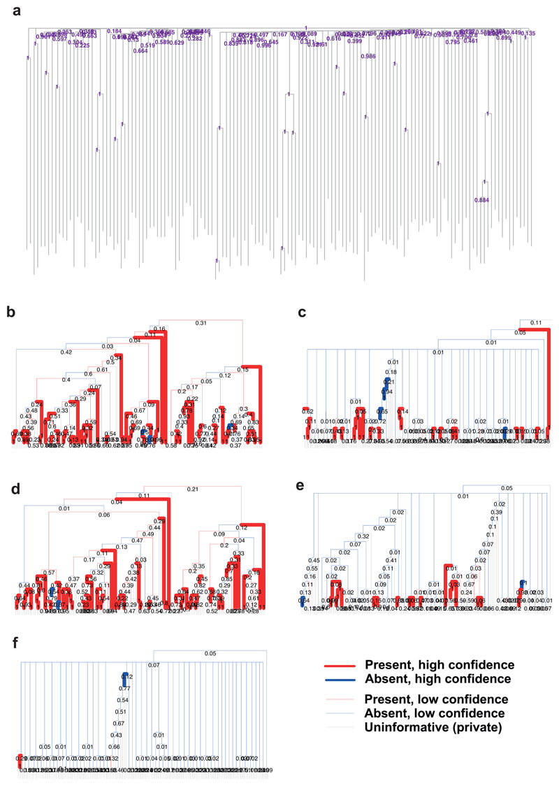
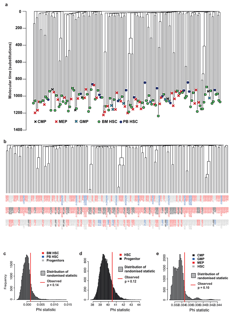
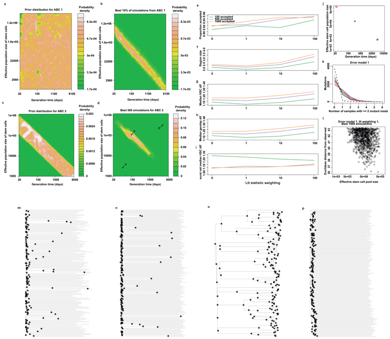
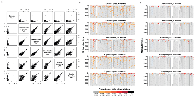
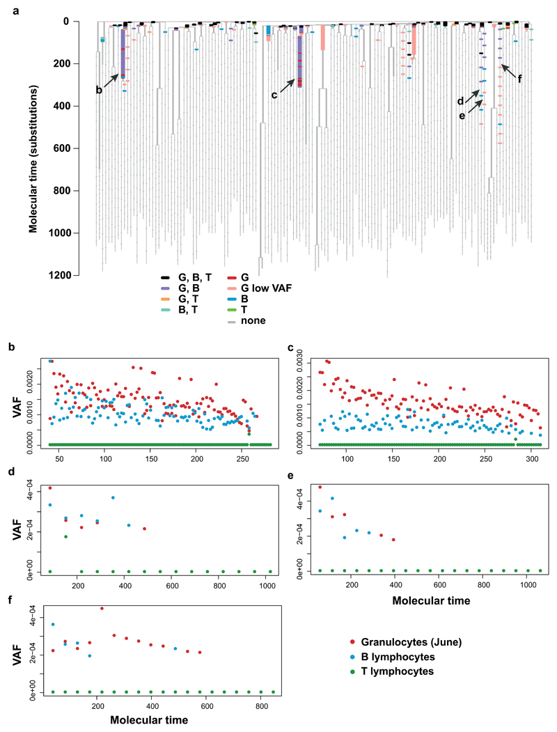
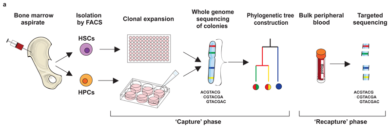
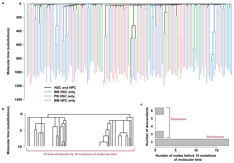
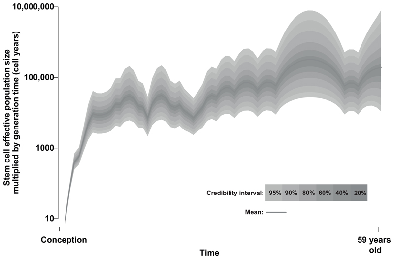
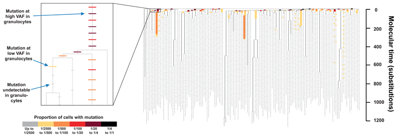
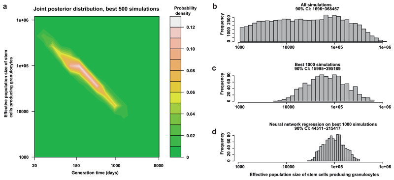
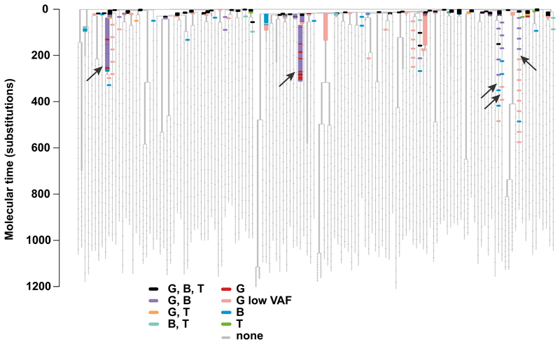
Haematopoietic stem cells drive blood production, but their population size and lifetime dynamics have not been quantified directly in humans. Here we identified 129,582 spontaneous, genome-wide somatic mutations in 140 single-cell-derived haematopoietic stem and progenitor colonies from a healthy 59-year-old man and applied population-genetics approaches to reconstruct clonal dynamics. Cell divisions from early embryogenesis were evident in the phylogenetic tree; all blood cells were derived from a common ancestor that preceded gastrulation. The size of the stem cell population grew steadily in early life, reaching a stable plateau by adolescence. We estimate the numbers of haematopoietic stem cells that are actively making white blood cells at any one time to be in the range of 50,000-200,000. We observed adult haematopoietic stem cell clones that generate multilineage outputs, including granulocytes and B lymphocytes. Harnessing naturally occurring mutations to report the clonal architecture of an organ enables the high-resolution reconstruction of somatic cell dynamics in humans.

Extended Figure 1. Cell sorting strategy.

(a) Sorting of stem and progenitor cells. Human bone marrow (BM) and peripheral blood (PB) mononuclear cells (time point 1) were stained with anti-CD34, anti-CD38, anti-CD45RA, anti-CD90, anti-CD10 and anti-CD135 antibodies. After exclusion of debris and doublets, gating on CD34, CD38 and CD90 were used to separate CD34+CD38-CD90+CD45RA-‘HSCs’. The CD34+CD38+ compartment was gated for CD10- cells before gating on CD135 (Flt3) and CD45RA to separate progenitor compartments: CD135+CD45RA ‘CMPs’, CD135+CD45RA+ ‘GMPs’ and CD135-CD45RA- ‘MEPs’. (b) sorting of B and T lymphocytes. PB mononuclear cells (time point +4 months) were stained with anti-CD4, anti-CD8 and anti-CD19 antibodies. After exclusion of debris and doublets, the CD4+CD8+CD19- gate was used to isolate T cells, while CD4-CD8-CD19+ gate was used to isolate B cells. (20,000 events shown). MEP: Megakaryocyte Erythrocyte Progenitor; CMP: Common Myeloid Progenitor; GMP: Granulocyte Macrophage Progenitor; HSC: Haematopoietic Stem Cell.

Extended Figure 2. Quality control of colonies as single-cell derived.

Example histograms of the variant allele fraction (VAF – the proportion of sequencing reads that report the mutation) of mutations in single colonies. (a) The VAF of all mutations on autosomes in a typical clonal colony. As there are two copies of each autosome, and each mutation occurs on only one of them, in a clonal sample the VAF of autosomal mutations is binomially distributed with mean 0.5. (b) The VAF of all mutations on the X chromosome in the same clonal colony. As our subject is male, there is only one copy of the X chromosome, and so true mutations here must have a VAF of 1. Occasionally, lower VAFs are seen due to the failure to detect a mutation on a read, or a read from another locus being aberrantly mapped to the locus in question and lowering the apparent coverage, or a mutation acquired in vitro. (c) and (d) show the VAF of autosomal and X chromosome mutations, respectively, in a typical colony seeded by more than one cell. As not all the reads come from the same cell, and most mutations are private to a given cell, a lower proportion of DNA molecules carry the mutation in a polyclonal colony than in a clonal colony, resulting in a leftward shift of the peak of the VAF histogram. These histograms suggest that the number of mutations acquired by the colonies in a few weeks of in vitro expansion is a small fraction of those acquired in vivo over 60 years of life.

Extended Figure 3. Mutation burden of colonies.

(a) A histogram of substitution (left hand panel) and indel (right hand panel) burden per colony. (b) The location around the genome of substitutions from all clones combined is shown as a circos plot. The outermost ring of the circos plot depicts the karyotypic ideogram. Moving inwards, base substitutions are shown as rainfall plots where the height of the dot in the substitution ring is proportional to log10 of the distance to the next mutation and with the colour of the dot illustrating the base change, as shown in the key. (c) a comparison of the substitution burden between stem cells (HSCs) and progenitor cells (HPCs). There were not significantly more mutations in progenitors than stem cells (p=0.14, Wilcoxon Rank Sum test).

Extended Figure 4. Trinucleotide context of mutations in normal blood colonies.

(a) The trinucleotide context of substitutions from all colonies combined. Substitutions can be classed according to the base change (referred to by the pyrimidine of the mutated base pair), and the bases 5’ and 3’ of the mutated one, into 96 categories. The counts in each of these categories is shown. (b) comparison with pooled acute myeloid leukaemia genomes, excluding genomes with >1500 mutations, and publicly available data on normal tissues that have been whole genome sequenced so far. The ordering of bars is the same as in panel a, and the same figure as in panel a is provided again at the same resolution for ease of comparison. Please note that these samples have been sequenced on different platforms using different systems, which is likely to result in small differences. Normal liver, normal colon, and normal small intestine were whole genome sequencing of single-cell derived organoids, whereas normal neurones were derived from single cells that had undergone whole genome amplification. (c) Example trinucleotide substitution plots for a selection of individual colonies derived from either stem cells (which have the prefix “BMH”) or progenitor cells (which have the prefix “BMP”). The ordering of bars is the same as in panel a.

Extended Figure 5. Construction of the phylogeny using different methods.

(a) The phylogeny of cells as presented in figures 2, 4, and 6, but with the addition of p values next to every node, derived by bootstrapping the substitution matrix 1000 times, building a tree using SCITE for each replicate, and counting the proportion of the bootstrapped trees that support each node. (b)-(f) Phylogenies constructed using different datasets and methods. In each case the phylogeny was constructed using 100 bootstraps of the data, and the p value for each node shown underneath it. Branches are coloured by whether a branch ancestral to exactly the same descendants is also present in the SCITE tree, and are drawn with a thicker line if the branch is recovered in >=70% of bootstrap replicates. (b) Substitution and indel datasets combined, building the tree by maximum parsimony. (c) Substitution, indel, and neighbour joining datsets combined, building the tree by neighbour joining. (d) Substitutions, tree build by maximum parsimony. (e) Indels, tree built by maximum parsimony. (f) Short tandem repeats, tree built by neighbour joining.

Extended Figure 6. Relationship between cell types in phylogeny.

(a) The phylogeny showing different stem and progenitor cell types. (b) The phylogeny is shown as in part (a), but with the labels underneath coloured by which cell types are being compared. The first row of labels has stem cells from bone marrow in red, progenitor cells from bone marrow in grey and stem cells from peripheral blood in black. The second row of labels has stem cells in red and bone marrow progenitors in black. The third row of labels has MEPs in red, CMPs in black, GMPs in blue and stem cells in grey. (c)-(e) Analysis of molecular variance (AMOVA) is used to test for clustering on the phylogeny for each of stem cells derived from peripheral blood vs bone marrow (c), stem cells vs progenitors (d), and different progenitor types (e). In each panel is shown the histogram of the null distribution of the statistic used to detect clustering, obtained by randomly permuting which cells are assigned to which category. Comparisons are only between cell types not shown in grey in panel (b). The observed value of the statistic is shown as a red vertical line. BM: bone marrow-derived; PB: peripheral blood-derived; HSC: haematopoietic stem cell; CMP: common myeloid progenitor; GMP: granulocyte macrophage progenitor; MEP: megakaryocyte erythrocyte progenitor.

Extended Figure 7. Approximate Bayesian Computations (ABC).

(a) The joint prior distribution for stem cell numbers (HSCs) and the generation time for the first ABC. (b) The location in sample space of the 10% of simulations that produced summary statistics (using only the ltt summary statistics – see methods and technical supplement) most similar to the observed summary statistics. (c) The joint prior distribution for the second ABC, in the area of sample space indicated to be plausible by the first set of simulations. (d) The joint posterior distribution of the best 500 simulations from the second ABC, as shown in figure 5 for ease of reference. Letters n, o, and p on the plot indicate the position in sample space from which panels (n), (o), and (p) were drawn, respectively. (e)-(i) Cross-validation of the model to choose the number of accepted simulations and the weighting applied to the ltt summary statistics (methods and technical supplement). (j) For illustrative purposes, five simulations were sampled for each of three population sizes along the plausible diagonal of sample space indicated in panel (b). One set of summary statistics are shown for these simulations in (k). Here, a red line indicates a simulation coming from the area of sample space indicated by a red point in (j); idem for blue and green lines. The black dotted line indicates the observed values for these summary statistics. This set of summary statistics counts, for different numbers of samples (x axis), how many of the 3952 mutations considered (y axis) are in this many samples with two or more reads, using error model 1 (which simulates errors according to the error rate in control DNA (supplementary methods)). The same summary statistics were calculated for different mutant read number cutoffs. (l) For each of the 1000 simulations that produce summary statistics most similar to the observed, the Euclidean distance from the observed (y axis) is plotted against the number of stem cells in that simulation (x axis). This information is used by the neural network regression step to define the most likely value for the number of stem cells. It can be seen that the most similar values are seen at around 100,000 stem cells, which was the location of the median of the posterior distribution from neural network regression. (m) The observed phylogeny, with branch points indicated by asterisks. (n)-(p) Phylogenies drawn from simulations that occur at the points in sample space indicated in panel (d). (n) represents a relatively plausible simulation, since the pattern of branch points is not dissimilar from that seen in the observed phylogeny (m). Simulations with smaller stem cell populations and faster stem cell turnover rates resulted in phylogenies where the stem cells are very closely related to each other (p), whereas those with larger populations and slower turnover result in phylogenies where the stem cells only share an embryonic common ancestor, and no branches are seen through the tree (p).

Extended Figure 8. Targeted sequencing data.

(a) Correlations between the variant allele fractions (VAFs) of all sequenced samples, shown on a log scale. Note that samples that were sequenced to lower depth cannot have VAFs as small as samples sequenced to higher depths. (b) Targeted sequencing information with no error correction. The data are shown as in figure 4 for all the samples interrogated, but just focusing on the first 350 mutations of molecular time. To allow a better comparison between samples sequenced at different depths, a higher detection threshold and different detection threshold are used relative to figure 4. (c) Targeted sequencing information after using cord blood controls for sequencing error correction with the Bayesian generalised poisson mixed effects model. The colour scale is the same as in panel b. The granulocytes 9 month timepoint is the same data as in figure 4 (provided again for ease of comparison), but plotted with a different colour scale.

Extended Figure 9. Multilineage clonal output

(a) The phylogeny with targeted sequencing information in different blood fractions overlaid as in Figure 6, shown again here for ease of reference. The colouring of mutations reflects which peripheral blood cell fractions they could be detected in, as indicated by the colour key. Arrows indicate adult clones with multilineage output, with letters corresponding to the panels below. G, granulocytes; G low VAF, granulocytes, allele fraction too low to be detected in lymphocytes; B, B lymphocytes; T, T lymphocytes. (b)-(f) Variant allele fractions of all mutations on branches (indicated by arrows in (a)) with mutations beyond molecular time 100 that are detectable in granulocytes and B lymphocytes but not T lymphocytes.

Figure 1. Experimental design.

The experiment proceeded in two phases: a ‘capture’ phase, in which single haematopoietic stem and progenitor cells were expanded in vitro and whole genome sequenced, and a ‘recapture’ phase, in which bulk populations of differentiated cells were deep sequenced for mutations identified in the capture phase. HSC, haematopoietic stem cell; HPC, haematopoietic progenitor cell; FACS, fluorescence activated cell sorting.

Figure 2. The phylogeny of cells, showing the relationship between cell types, and embryological cell divisions.

(a), phylogeny of 140 single haematopoietic stem and progenitor cells showing the relationship between cell types. At each tip of the tree is a colony. Branches connect colonies to each other to form a family tree. Branch lengths are proportional to the number of somatic mutations. Branches are coloured according to the phenotype of their descendants. Branches ancestral to haematopoietic progenitor cells (HPCs) are coloured red, branches ancestral to bone marrow-derived haematopoietic stem cells (BM HSCs) blue, and branches ancestral to peripheral blood-derived haematopoietic stem cells (PB HSCs) green. Branches ancestral to both stem and progenitor cells are coloured black. (b) the same phylogeny as in figure 2a, but showing only the first 10 mutations of molecular time. (c) the number of descendants of each node for the first 10 mutations of molecular time, used to estimate the embryonic mutation rate.

Figure 3. Population size trajectory of stem cell pool.

Phylodynamic methods reveal changes in the effective population size of stem cells over life based on the timing of coalescences (branch-points) in our observed phylogeny. Shading illustrates different credibility intervals. The y axis is shown in units of ‘population size multiplied by generation time’ (cell-years) because the same distribution of coalescences can be generated from a population of 10 times the size with 10 times as many generations.

Figure 4. ‘Recapture’ of mutations by targeted sequencing.

The phylogenetic tree of cells is shown as in Figure 2, but information from targeted sequencing of peripheral blood granulocytes from the 9 month time-point is overlaid. This is shown more clearly in the inset, which zooms in on a portion of the tree. The underlying structure of the tree is shown in grey. On top are placed horizontal bars, one for every mutation in the bait-set for targeted sequencing. Bars are coloured according the proportion of cells in the sample that carry the mutations (obtained by multiplying the variant allele fraction for autosomal mutations by two), indicated in the colour scale. Undetectable mutations are coloured grey and shown as smaller bars. Mutations have been spaced evenly along a branch according to their mean variant allele fraction from targeted sequencing of all granulocyte and lymphocyte time-points combined. A higher density of baits were designed for branches shared by more than one colony. On these branches the mutations are so close together that they can appear as one continuous bar.

Figure 5. Approximate Bayesian computation (ABC) of the number of stem cells and their replication rate.

(a) A contour plot of the most likely values for stem cell numbers and time between symmetrical stem cell divisions over the sample space that was simulated. It shows the stem cell number and generation times of the 500 simulations that produced summary statistics that were most similar to the summary statistics extracted from the observed data. (b) The prior distribution for the number of stem cells contributing to granulocytes for the second ABC (i.e. the stem cell numbers for all 80,000 simulations). (c) The distribution of stem cell numbers for the 1000 simulations that produced summary statistics most similar to the observed summary statistics. (d) The posterior distribution of a neural network regression run on these 1000 simulations. The 90% credibility interval is quoted for the stem cell population in each of (b)-(d).

Figure 6. Targeted sequencing of granulocyte and lymphocyte samples.

The phylogeny is depicted as in Figure 4, with the underlying structure of the tree shown in grey, and horizontal bars drawn to represent every mutation in the bait-set. Here the colouring of mutations reflects which peripheral blood cell fractions they could be detected in, as indicated by the colour key. Two colours are used for granulocytes: red for mutations only detected in granulocytes that were are at a sufficiently high allele fraction to have been found in the shallower lymphocyte sequencing data and pink for mutations that were only detected in granulocytes, but at such a low allele fraction (<1/2000 reads) that if they had been present in lymphocytes at this allele fraction they would not have been detected. Arrows indicate adult clones with multilineage output. G, granulocytes; B, B lymphocytes; T, T lymphocytes.

References

1. Till JE, McCulloch EA. A direct measurement of the radiation sensitivity of normal mouse bone marrow cells. Radiat Res. 1961;14:213–22. - PubMed
1. Becker AJ, McCulloch EA, Till JE. Cytological demonstration of the clonal nature of spleen colonies derived from transplanted mouse marrow cells. Nature. 1963;197:452–4. - PubMed
1. Lemischka IR, Raulet DH, Mulligan RC. Developmental potential and dynamic behavior of hematopoietic stem cells. Cell. 1986;45:917–27. - PubMed
1. Antoniou AC, et al. Breast-Cancer Risk in Families with Mutations in PALB2. N Engl J Med. 2014;371:497–506. - PMC - PubMed
1. Naik SH, et al. Diverse and heritable lineage imprinting of early haematopoietic progenitors. Nature. 2013;496:229–32. - PubMed