New tools for the analysis and validation of cryo-EM maps and atomic models

Abstract

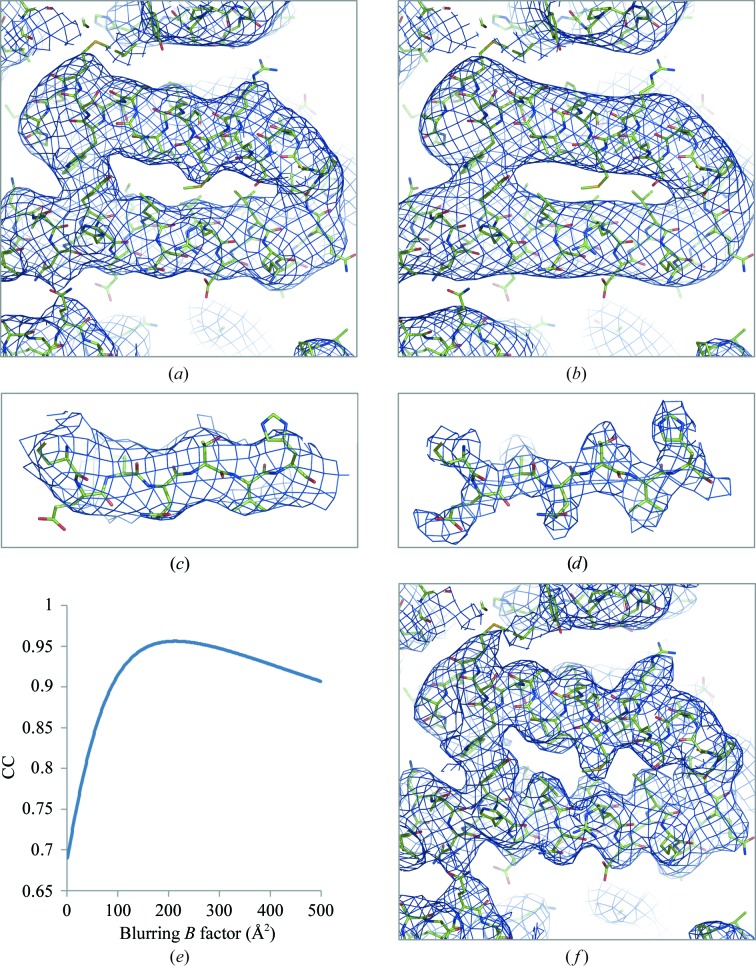
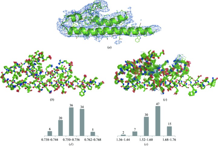
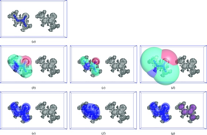
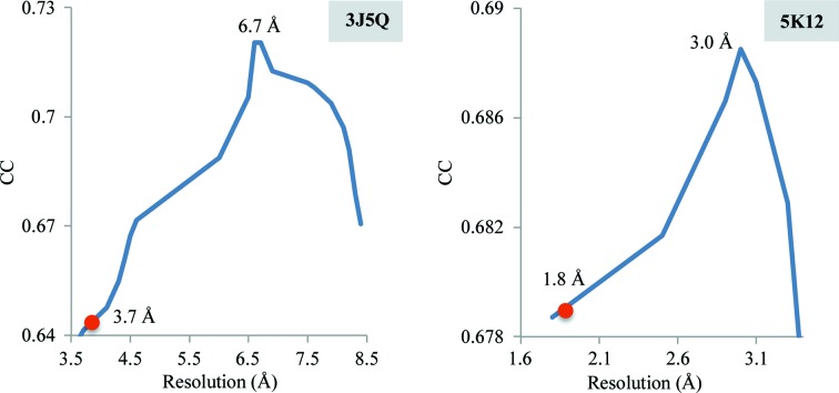
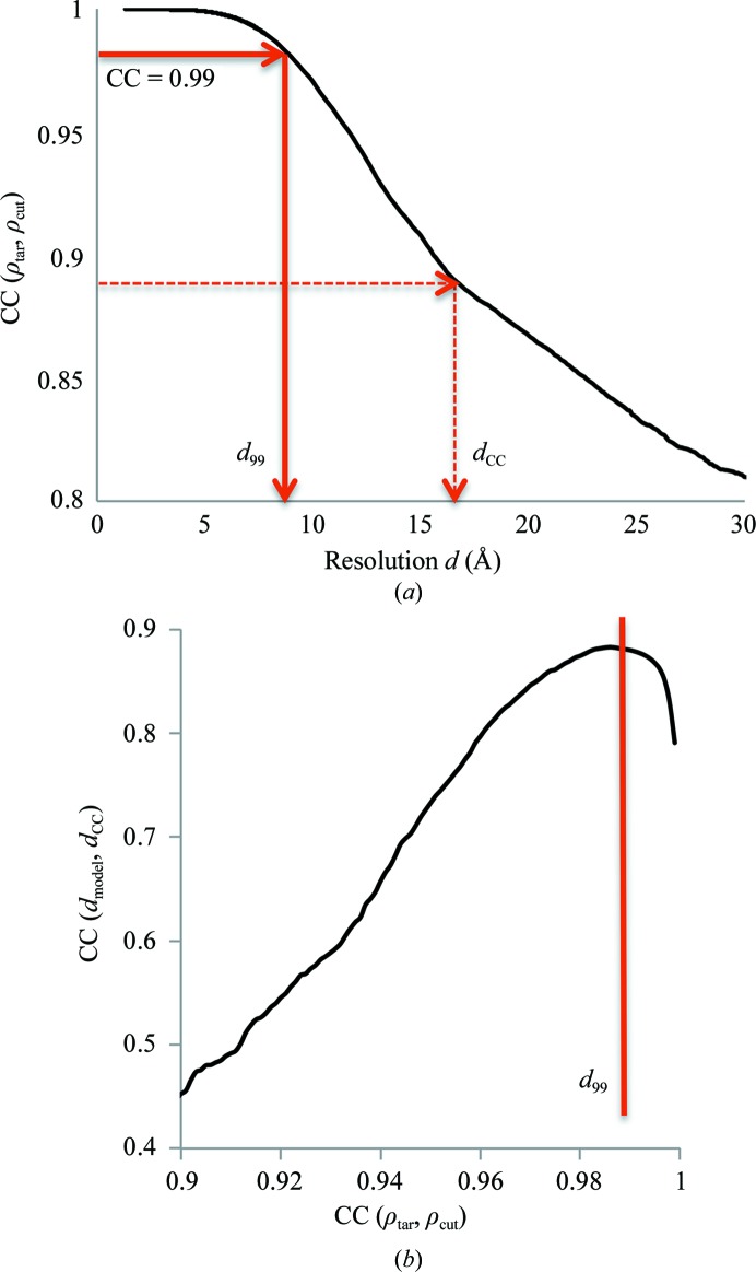
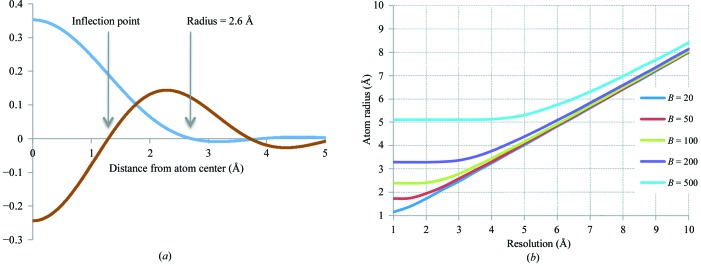
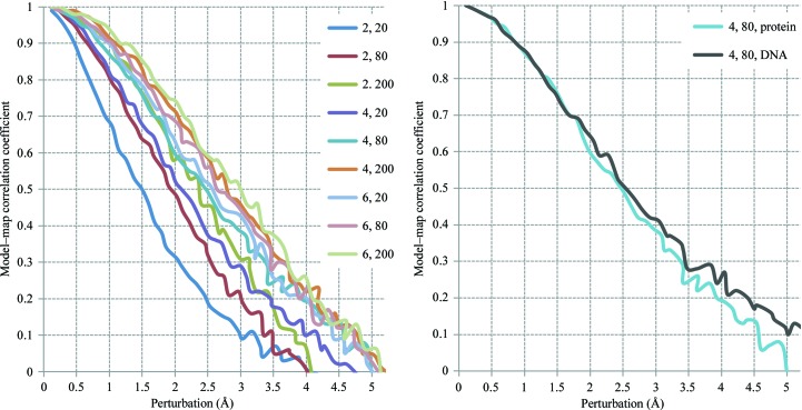
Recent advances in the field of electron cryomicroscopy (cryo-EM) have resulted in a rapidly increasing number of atomic models of biomacromolecules that have been solved using this technique and deposited in the Protein Data Bank and the Electron Microscopy Data Bank. Similar to macromolecular crystallography, validation tools for these models and maps are required. While some of these validation tools may be borrowed from crystallography, new methods specifically designed for cryo-EM validation are required. Here, new computational methods and tools implemented in PHENIX are discussed, including d₉₉ to estimate resolution, phenix.auto_sharpen to improve maps and phenix.mtriage to analyze cryo-EM maps. It is suggested that cryo-EM half-maps and masks should be deposited to facilitate the evaluation and validation of cryo-EM-derived atomic models and maps. The application of these tools to deposited cryo-EM atomic models and maps is also presented.

Keywords: atomic models; cryo-EM; data quality; model quality; resolution; validation.

Figure 1

Cryo-EM models in the PDB. (a) Cumulative number of models and (b) mean resolution extracted from the database by year. (c) Distribution of the resolution for all models.

Figure 2

Model-geometry metrics for models at 4.5 Å resolution or better. The number at the top of each bar shows the percentage of structures that fall into the category. x axis: percentages of outliers (rotamer, Ramachandran and C^β deviation) and clashscore value. Curves show by-year average percentages of Ramachandran, rotamer and C^β deviation outliers, as well as values of clashscore. For clarity in presentation, the percentages of rotamer and Ramachandran plot outliers are scaled by 1/3 and the clashscore is scaled by 1/10.

Figure 3

Examples of problematic secondary-structure (SS) annotations shown as pairs of cartoon representation and corresponding Ramachandran plot. (a) The α-helix looks plausible although slightly distorted, but most residues are Ramachandran plot outliers. (b) The α-helix is obviously distorted; there are no Ramachandran plot outliers, but only one angle belongs to the α-­helix region of the plot. (c) Distorted α-helix with all but one residue belonging to the expected Ramachandran plot region. (d) Apparently two α-helices annotated as one with many (φ, ψ) pairs being out of the α-helix region.

Figure 4

Distribution of all four correlation measures (CCs) considered in this work, CC_box, CC_mask, CC_volume and CC_peaks, for models at 4.5 Å resolution or better; values (a) below 0.5 and (b) above 0.5 are shown separately for clarity. (c) Comparison of CC_mask calculated using the original maps and the same maps sharpened with phenix.auto_sharpen (resolution 4.5 Å or better). The overall CC_mask averages are 0.676 and 0.665 using the original and sharpened maps, respectively.

Figure 5

Distribution of CC_mask versus CC_volume (a) and CC_box versus CC_peaks (b) for entries at a resolution of 4.5 Å or better.

Figure 6

Model and map (PDB and EMDB codes 3J9E and 6240, respectively; resolution 3.3 Å) showing some parts of the model that do not fit the map at any chosen threshold contouring level (shown in red).

Figure 7

Model and map (PDB and EMDB codes 6CRZ and 7577, respectively; resolution 3.3 Å) showing a combination of two issues. (a) Some parts of the model do not fit the map. (c, d, e) Improvements that can be achieved after a round of refinement using phenix.real_space_refine: compare the model-to-map fit before (red) and after (black) refinement. (b) Model–map correlation CC_mask shown per residue: red and black are before and after refinement, respectively.

Figure 8

(a, c) An apparently over-sharpened map (PDB and EMDB codes 5NV3 and 3699, respectively; resolution 3.39 Å). Applying phenix.auto_sharpen improves the map by blurring it. (b, d) Subsequent refinement against the blurred map improves the model-to-map fit, as shown by CC_mask reported per residue (e) (black dots).

Figure 9

Scatter plots showing the relationship between the different resolution estimates and their different ways of calculation. (a) d _FSC calculated using original half-maps versus d _FSC using sharpened half-maps; a mask was used in both cases. As expected, d _FSC is essentially insensitive to map sharpening. (b) Comparison of d _FSC extracted from the EMDB (referred to as d _EMDB) with recalculated values using available half-maps with masking applied (red) and not applied (blue); no sharpening was used in both cases. (c) d _{FSC_model} calculated at FSC 0 (red), 0.143 (blue) and 0.5 (green) versus d _FSC from available half-maps (using a mask, no sharpening). The correlation CC(d _FSC, d _{FSC_model}) is 0.929, 0.959 and 0.973 for FSC thresholds at 0.5, 0 and 0.143, respectively. (d) d _model versus d _FSC calculated using original half-maps (no sharpening). The correlation is rather marked, but clearly d _model shows lower resolution, likely owing to smearing by atomic displacement parameters. (e) d ₉₉ calculated using the original (no sharpening) masked map versus d _FSC calculated using the original half-maps (no sharpening). (f) d _{FSC_model} calculated with and without masking (taken at FSC = 0.143). Clearly, this resolution metric is not sensitive to using a mask. (g) d ₉₉ calculated using original and sharpened maps (masking was used in both cases). Since map attenuation performed using phenix.auto_sharpen can sharpen or blur the map, the d ₉₉ value can be smaller or larger, depending on whether blurring or sharpening occurred. (h) d ₉₉ calculated using a masked map and an unmasked map (no sharpening in both cases). Since masking eliminates the noise outside the molecular region, d ₉₉ calculated without masking results in systematically smaller values.

Figure 10

Maps for PDB entry 5UAR calculated by consecutive execution of the following steps: Fourier transform the original experimental map (EMDB code 8461), select a subset of Fourier coefficients of specified resolution range and finally calculate the new map using selected coefficients. Resolution ranges in Å: (a, c) 1.9–∞, (b, d) 6.7–∞, (e) 1.9–3.3, (f) 3.3–6.7. Pairs of maps (a, b) and (c, d) are the same maps shown at different contouring thresholds: high and low, respectively.

Figure 11

Sharpened maps for PDB entry 5UAR calculated similarly to as in Fig. 10 ▸ using data in the resolution ranges (a) 3.3–∞ Å (B = −240 Ų) and (b) 1.9–∞ Å (B = −20 Ų).

Figure 12

Maps for PDB entry 5LDF. (a) and (b) are shown with a low and high contouring threshold, respectively. (c) Fragment of a well resolved chain from a relatively high-resolution region, showing some side chains typical for resolutions of 4–4.5 Å (chain B, residues 435–460).

Figure 13

Maps for PDB entry 5K12 in the resolution ranges (a) 1.8–∞ Å, (b) 3–∞ Å, (c) 1.8–∞ Å sharpened with B = −35 Ų and (d) 2.3–∞ Å sharpened with B = −38 Ų. Residue 382 in chain A is shown.

Figure 14

Maps for PDB entry 5K7L: (a) original and (b) calculated using Fourier map coefficients in the 7.4–∞ Å resolution range. (c) The original map and (d) the map calculated using 3.6–7.4 Å resolution data are shown for residues 568–574. (e) Correlation between 7.4 Å resolution and overall B-­factor-blurred 3.8 Å resolution model-calculated maps as a function of blurring B-factor. (f) Sharpened original map.

Figure 15

Illustration of multiple interpretation. (a) PDB entry 3J0R and the corresponding map (EMDB code 5352). (b) Ensemble of 100 perturbed models obtained using MD; all models in the ensemble deviate from the starting model by 0.5 Å. (c) Real-space refined models obtained from (b) using phenix.real_space_refine. (d) Distribution of model–map correlation for refined models. (e) Distribution of r.m.s. deviations between starting and refined models.

Figure 16

Illustration of different subsets of the grid nodes used to calculate the correlation coefficients between model and target maps. (a) Atomic model (blue sticks) superposed with partially interpreted target map (gray); the correlation coefficient CC_box between the target and model map is calculated over the whole cell. (b) Molecular mask calculated by Jiang & Brünger (1994 ▸), CC_mask. (c, d) Mask derived from atomic images at higher and lower resolutions, CC_image. (e, f) Peaks within the given volume in higher and lower resolution model maps CC_volume. (g) Mask derived from the peaks of the model (blue) and target (magenta) maps, CC_peaks; the total mask is the union of the blue and magenta masks.

Figure 17

Correlation coefficient between an experimental map and maps generated from the model at different resolutions, shown for selected PDB entries. The red circle on each curve indicates the reported resolution, d _FSC, and the number on the top of the peak indicates the estimated resolution.

Figure 18

(a) Correlation coefficient [equation (4), Appendix C ] between the original map and a high-resolution truncated map shown as a function of the resolution value used for truncation for PDB entry 3J27. d ₉₉ corresponds to CC = 0.99. (b) Correlation coefficient between d _model and trial resolution cutoffs d _CC, calculated using all selected data sets, shown as function of CC(ρ_tar, ρ_cut). See Appendix C for details.

Figure 19

(a) 3 Å resolution Fourier image of a C atom with B factor 50 Ų (blue) and its second derivative (brown); the image is spherically symmetric and is represented by a one-dimensional radial distribution. The atom radius is defined as twice the distance from the center of the atom to the first inflection point of this curve. (b) Radius as determined in (a) for the C atom as a function of resolution, shown for several B-factor values.

Figure 20

Model–map correlation coefficient calculated between a target map and the map from a perturbed model shown as function of perturbation at different resolutions (2, 4 and 6 Å) and different overall ADPs (20, 80 and 200 Ų). Left, a protein model. Right, copy of a curve for the protein model taken from the left picture (light blue) and the corresponding curve obtained at the same resolution and ADP for an RNA molecule; this illustrates the low dependence of the results on the choice of molecule.

References

1. Adams, P. D. et al. (2010). Acta Cryst. D66, 213–221. - PubMed
1. Afanasyev, P., Seer-Linnemayr, C., Ravelli, R. B. G., Matadeen, R., De Carlo, S., Alewijnse, B., Portugal, R. V., Pannu, N. S., Schatz, M. & van Heel, M. (2017). IUCrJ, 4, 678–694. - PMC - PubMed
1. Afonine, P. V., Grosse-Kunstleve, R. W., Adams, P. D. & Urzhumtsev, A. (2013). Acta Cryst. D69, 625–634. - PMC - PubMed
1. Afonine, P. V., Grosse-Kunstleve, R. W., Chen, V. B., Headd, J. J., Moriarty, N. W., Richardson, J. S., Richardson, D. C., Urzhumtsev, A., Zwart, P. H. & Adams, P. D. (2010). J. Appl. Cryst. 43, 669–676. - PMC - PubMed
1. Afonine, P. V., Headd, J. J., Terwilliger, T. C. & Adams, P. D. (2013). Comput. Crystallogr. Newsl. 4, 43–44.