. 2018 Sep 10;373(1758):20170377.
doi: 10.1098/rstb.2017.0377.

Functional connectomics from neural dynamics: probabilistic graphical models for neuronal network of Caenorhabditis elegans

Affiliations

Functional connectomics from neural dynamics: probabilistic graphical models for neuronal network of Caenorhabditis elegans

Hexuan Liu et al. Philos Trans R Soc Lond B Biol Sci. .

Abstract

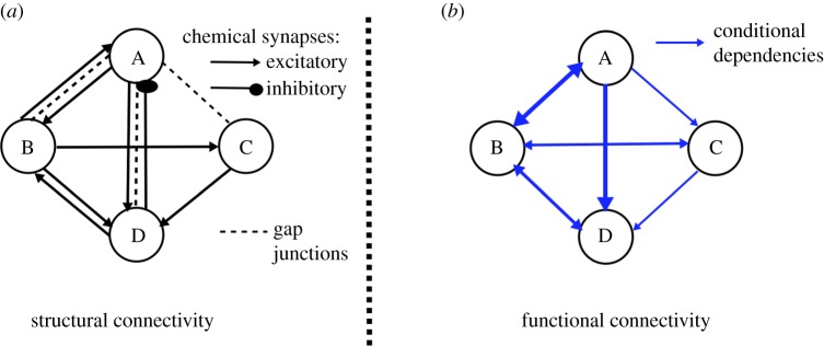
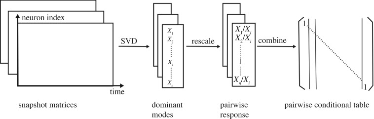
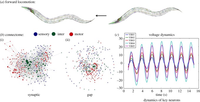
We propose an approach to represent neuronal network dynamics as a probabilistic graphical model (PGM). To construct the PGM, we collect time series of neuronal responses produced by the neuronal network and use singular value decomposition to obtain a low-dimensional projection of the time-series data. We then extract dominant patterns from the projections to get pairwise dependency information and create a graphical model for the full network. The outcome model is a functional connectome that captures how stimuli propagate through the network and thus represents causal dependencies between neurons and stimuli. We apply our methodology to a model of the Caenorhabditis elegans somatic nervous system to validate and show an example of our approach. The structure and dynamics of the C. elegans nervous system are well studied and a model that generates neuronal responses is available. The resulting PGM enables us to obtain and verify underlying neuronal pathways for known behavioural scenarios and detect possible pathways for novel scenarios.This article is part of a discussion meeting issue 'Connectome to behaviour: modelling C. elegans at cellular resolution'.

Keywords: Caenorhabditis elegans; functional connectome; neuronal networks; probabilistic graphical models.


Conflict of interest statement

We declare we have no competing interests.

Figures

Figure 1.
Figure 1.
Representation of a neuronal network as a graphical model. (a) Example of structural/anatomical connectivity map in which nodes denote neurons and edges map connections, e.g. chemical synapses and electrical gap junctions. Interactions between neurons produce a nonlinear network that dynamically transports stimuli to neuronal behaviours. (b) Example of PGM constructed from the neuronal network governed by the structural connectivity map and nonlinear dynamics. In the PGM, nodes are random variables corresponding to neuronal states and edges are conditional probabilities. PGM structure captures functionality of the network and hence is typically different from the anatomical connectivity map. (Online version in colour.)
Figure 2.
Figure 2.
Construction of dependencies between nodes. By injecting input stimuli into each neuron, we obtain a series of snapshot matrices that record network dynamics. By decomposing the snapshot matrices using SVD, we obtain the decomposition modes and compress them into a single vector for each matrix. We then normalize the vector according to its input neuron and obtain pairwise responses, which constitute the adjacency matrix of pairwise conditional probabilities.
Figure 3.
Figure 3.
Tree construction from adjacency matrices. We start with the input node, and sort the other nodes according to their probabilities conditioned on the input node. We ignore nodes with conditional probabilities lower than the threshold, and select the top nodes with the highest conditional probabilities. A constraint can be imposed to limit the number of children that a node can have. From there we extend each node recursively, until it either reaches the maximum tree depth, or reaches neurons in a particular set (e.g. motor neurons). The threshold, maximum tree depth and maximum number of children are pre-set parameters to limit the size of the tree.
Figure 4.
Figure 4.
Construction of PGMs for three-unit motifs. (a) Connectomes of four examined motifs. (b) Network responses when external input is injected into each unit (indicated by diagonal arrow). The colour of the units indicate the activation level of each unit, i.e. darker colour indicates a more active node. (c) Constructed PGM structures. If there is an edge from X to Y, then the conditional probability P(Y | X) > 0.1. Stronger arrows correspond to higher probability.
Figure 5.
Figure 5.
Two layers of the neuronal network of C. elegans. (a) An example of forward locomotion induced by two layers of the neuronal network of the worm (image credit http://www.connectomeengine.com/). The first layer (b): connectome of C. elegans, consisting of 297 somatic neurons, 6393 chemical synapses and 890 gap junctions. The connectome shows (i) the chemical synapses between neurons and (ii) the gap junctions. The second layer (c): neural dynamics modelled by differential equations. Here, we show voltage oscillations of the motor VB group. Combining the two layers we achieve the dynome, a dynamically evolving network, which is the foundation for constructing the PGM.
Figure 6.
Figure 6.
Top connected neurons in sensory, inter and motor groups. (ac) We compare three groups: functional connectivity represented by PGM, connectome mapping chemical synapses, and a connectome mapping gap junction. Connectivity is measured by the number of incoming edges. Top five connected neurons in each group along with the number of incoming edges into them are shown. In the synaptic group, an edge exists from one node (Xi) to another (Xj) if there is at least one chemical synapse XiXj. In the gap group, an edge exists between Xi and Xj when there is at least one gap junction between Xi and Xj, as the gap junctions are non-directed. In the PGM group, an edge exists from Xi to Xj if P(Y = 1|X = 1) > threshold, set here as threshold = 0.1. (d) Number of incoming edges in the PGM for ASJ and ASK sensory neurons, categorized into three classes (sensory, inter and motor).
Figure 7.
Figure 7.
Connectivity matrices of gap, synaptic and PGM. In the dependency matrices, the element in the jth column and ith row, aji, represents the total number of gap contacts/synaptic contacts, probability dependencies respectively from ith neuron to jth neuron. The subplots motor formula image sensory, motor formula image motor, sensoryformula image 
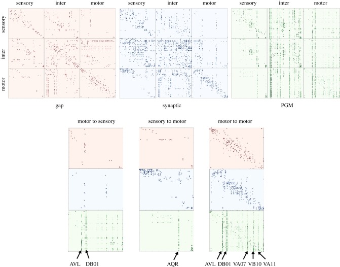
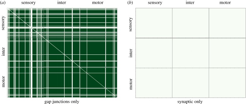
motor are zoomed in to compare detailed differences in gap, synaptic and PGM connections. Input neurons that activate the majority of the responding neurons are labelled.
Figure 8.
Figure 8.
Sub-circuits that lead to forward and backward locomotion in C. elegans (a) Experimentally proposed connectome sub-circuit of forward and backward locomotion (sensory neurons are shown by rectangles, inter neurons by circles and motor neurons by triangles: FWD, forward; REV, reverse). Lines with arrows refer to chemical synapses and dashed lines refer to gap junctions. Reproduced from [18]. (b) Sub-circuits inferred from PGM. (i) Forward locomotion induced by injecting input into sensory neurons PLML and PLMR, known to trigger forward locomotion upon posterior touch. (ii) Backward locomotion induced by injecting input into ALML and ALMR, known to trigger backward locomotion upon anterior touch. (Online version in colour.)
Figure 9.
Figure 9.
MAP posterior inference: reverse tracking of A and B motor groups associated with locomotion. We identify a group of neurons using MAP inference. Given that a specific group of motor neurons are being excited, the set of inter and sensory neurons that leads to such excitation is shown. From top to bottom is the natural stimulus flow, i.e. sensory → inter → motor. From bottom to top is MAP inference. (Online version in colour.)
Figure 10.
Figure 10.
PGM dependency matrices constructed by including a single anatomical connectome (a: gap; b: synaptic) in the neural dynamics simulator. (Online version in colour.)

Similar articles

Cited by

References

    1. Koller D, Friedman N, Getoor L, Taskar B. 2007. Graphical models in a nutshell. In Introduction to statistical relational learning, pp. 13–55. Cambridge, MA: MIT press.
    1. Koller D, Friedman N. 2009. Probabilistic graphical models: principles and techniques. Cambridge, MA: MIT Press.
    1. Murphy KP. 2012. Machine learning: a probabilistic perspective. Cambridge, MA: MIT Press.
    1. Friedman N, Linial M, Nachman I, Pe'er D. 2000. Using Bayesian networks to analyze expression data. J. Comput. Biol. 7, 601–620. (10.1089/106652700750050961) - DOI - PubMed
    1. Kolar M, Song L, Ahmed A, Xing EP. 2010. Estimating time-varying networks. Ann. Appl. Stat. 4, 94–123. (10.1214/09-aoas308) - DOI

Publication types

LinkOut - more resources