Experimental and computational framework for a dynamic protein atlas of human cell division

Abstract

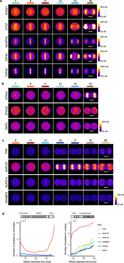
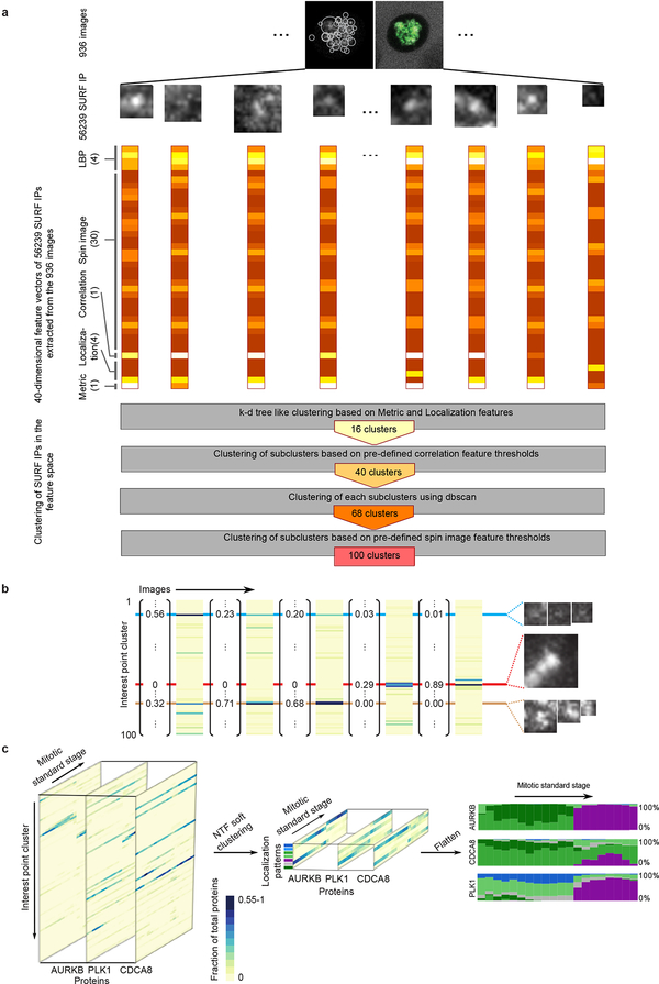
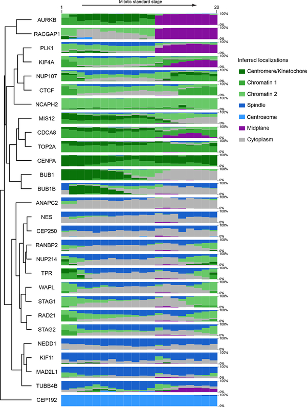
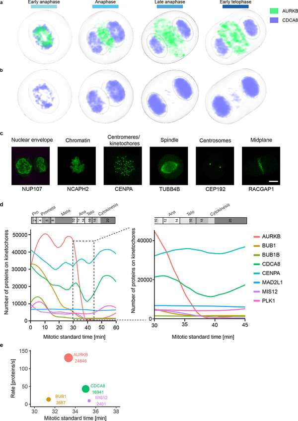
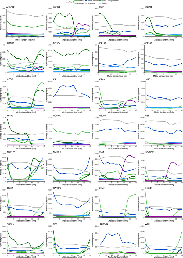
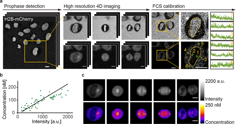
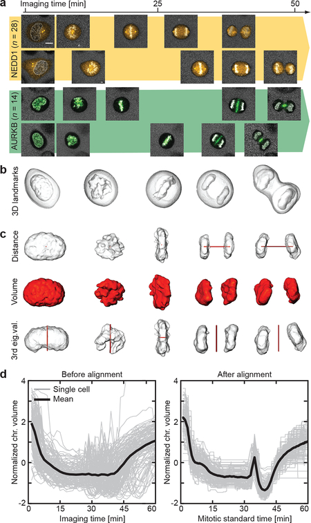
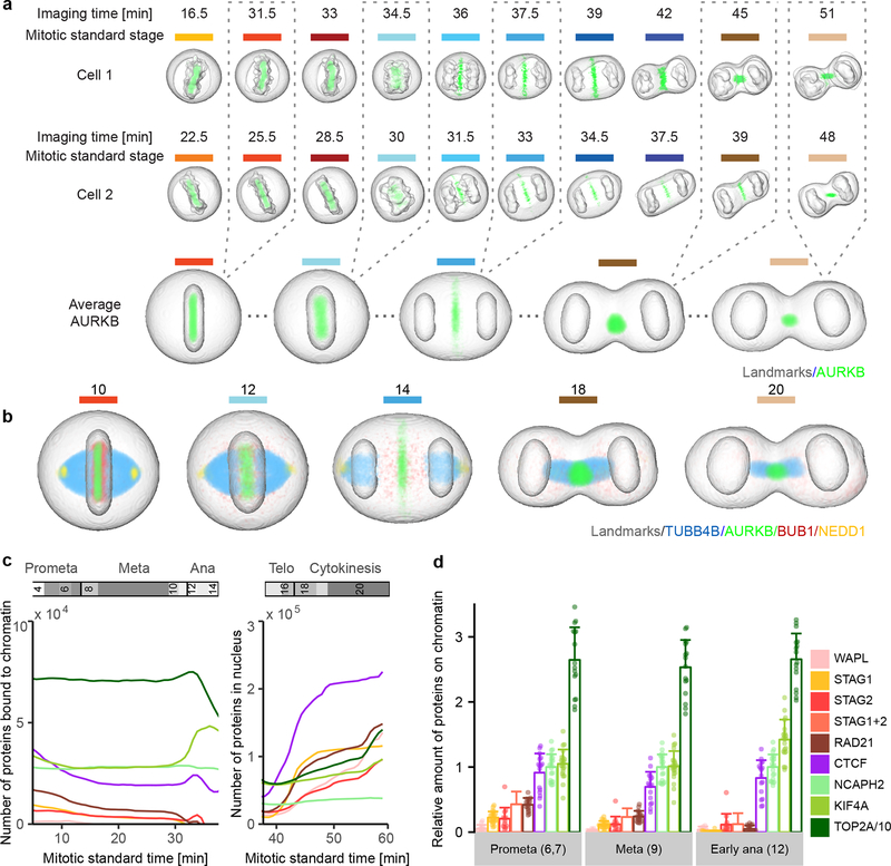
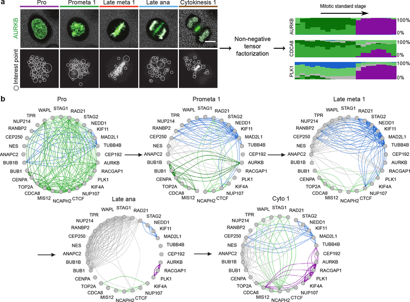
Essential biological functions, such as mitosis, require tight coordination of hundreds of proteins in space and time. Localization, the timing of interactions and changes in cellular structure are all crucial to ensure the correct assembly, function and regulation of protein complexes^1-4. Imaging of live cells can reveal protein distributions and dynamics but experimental and theoretical challenges have prevented the collection of quantitative data, which are necessary for the formulation of a model of mitosis that comprehensively integrates information and enables the analysis of the dynamic interactions between the molecular parts of the mitotic machinery within changing cellular boundaries. Here we generate a canonical model of the morphological changes during the mitotic progression of human cells on the basis of four-dimensional image data. We use this model to integrate dynamic three-dimensional concentration data of many fluorescently knocked-in mitotic proteins, imaged by fluorescence correlation spectroscopy-calibrated microscopy⁵. The approach taken here to generate a dynamic protein atlas of human cell division is generic; it can be applied to systematically map and mine dynamic protein localization networks that drive cell division in different cell types, and can be conceptually transferred to other cellular functions.

Extended Data Fig. 1 |

Segmentation and time alignment. (a-b) Segmentation and 3D reconstruction of landmarks. (a) Single x-y plane image in mCherry (587 – 621 nm, first row) and DY481XL (622 – 695 nm, second row) detection channels. Third row: detected chromatin markers where boundaries of the chromosomal volume of interest are marked in red. Fourth row: output of watershed transform on ratio image where boundary of the detected cell of interest is marked in green. Scale bar: 10 μm. (b) Reconstruction of cell and chromosomal surfaces in 3D (grey) and the predicted division axis (red). (c-e) Generating the mitotic standard time model. (c) Dynamic time warping is used to align a pair of time-resolved sequences. (d) Modified Barton-Sternberg algorithm to align 132 sequences. (e) The cumulative standard deviation of a single feature after each iteration of the algorithm. It remains nearly constant after the 2^nd round indicating that at termination (4^th round) a stable time alignment was achieved. This has been repeated 10 times and similar alignment results are obtained when the number of cells is more than 50.

Extended Data Fig. 2 |

Detection of mitotic standard stages. (a) Detection of major mitotic transitions of the mitotic standard time. Peaks in the second derivatives (red circles) above a pre-defined threshold (grey lines) were detected in all feature dimensions as mitotic transitions. (b) Additional smaller peaks (blue circles) were detected to ensure a maximum duration of 12 minutes for each standard stage. (c) Transitions were deleted (grey circles) such that all stages had a minimal duration of 1.5 minutes. (d) The standard mitotic cell was represented by the cell closest to the average of each stage. Each mitotic stage was assigned duration (colored line), its duration standard deviation (grey line) and a biological annotation.

Extended Data Fig. 3 |

Comparison between mitotic standard time for HeLa Kyoto and U2OS cells. (a) Features used for generating the mitotic standard time model after alignment for HeLa Kyoto cells (left column) and U2OS cells (right column). Grey line: normalized feature value over time of individual cells. Black line: average. (b) Mitotic standard time transitions for HeLa cells (left panel) and U2OS cells (right panel). (c) Standard mitotic U2OS cell represented by the cell closest to the average of each mitotic standard stage. Each mitotic stage was assigned duration (colored line), its duration standard deviation (grey line) and a biological annotation.

Extended Data Fig. 4 |

Generation of spatial model for standard mitotic stages by combining two cylindrical representations. Examples of cells in mitotic stage no. 10 (a) were registered using the predicted cell division axis as shown in (b). (c) Transformation between Cartesian and cylindrical coordinate systems. (d) Example cellular and chromosomal surfaces (grey) were transformed into the cylindrical coordinate system using two cylindrical axes (z-axis or predicted division axis) marked in yellow. (e) Average cellular and chromosomal surfaces in cylindrical coordinate systems. (f) Union (U) and intersection (∩) of the averaged landmarks volumes represented in the Cartesian coordinate system that were then combined to generate final cellular and chromosomal surfaces shown in the first image in (g). By averaging a large number of cells, models were generated for all mitotic standard stages with symmetrical geometries and example stages 10, 14, 16 and 19 are shown in (g). (h) The spatial variation of the mitotic standard spaces shown in (g).

Extended Data Fig. 5 |

Chromatin remodelers and NUPs localization. (a-c) Maximal intensity projection from the mitotic standard model at selected stages. Scale bars: 10 μm. (a) Chromatin remodelers RAD21, CTCF, NCAPH2, KIF4A and TOP2A present on chromatin during mitosis. (b) Chromatin remodelers with weak binding to chromatin during mitosis STAG1, STAG2, and WAPL. (c) Four NUPs at selected standard mitotic stages. (d) NUPs localization as function of mitotic standard time. The curves for STAG2 and WAPL are shown as a reference and are identical to the data from Fig. 3c.

Extended Data Fig. 6 |

Interest point clusters and dynamic protein localization. (a) Pipeline for the definition of interest point clusters using a subset of the data. 936 images (corresponding to 5 % of the entire data set) were randomly selected from the dataset to construct a pool of interest points. Each interest point was numerically described with a 40 dimensional feature vector encoding the intensity distribution, localization and contrasts to the interest point neighborhood. Combining k-d-tree-like and thresholding-based clustering with density based clustering, the interest points were grouped into 100 clusters. (b) The remaining interest points of the data set were then assigned to the identified clusters. Thus each image was represented as the distribution of intensity in each of the 100 interest point clusters. (c) Non-negative factorization of the data tensor of proteins × features × mitotic stages (left panel) produced a non-negative tensor of reduced dimension (middle panel) whose entries can be interpreted as the fraction of protein belonging to each cluster over time (right panel, each cluster is represented by a different color and the height of a colored bar at a given mitotic stage represents the fraction of the protein in the corresponding cluster at this stage).

Extended Data Fig. 7 |

Quantitative evolution of protein subcellular localizations inferred from non-negative tensor factorization of the proteins × features × time tensor. Each subcellular localization cluster was assigned a different color and named using known information on proteins belonging to that cluster. The height of each color band at each time point is proportional to the fraction of the protein amount in the corresponding cluster at that time point. Genes were grouped by complete linkage clustering followed by optimal leaf ordering.

Extended Data Fig. 8 |

Mitotic standard model and supervised classification to investigate the dynamic localization of kinetochore proteins. (a-b) Concentration maps of chromosome passenger complex proteins AURKB and CDCA8 in anaphase and early telophase. (a) AURKB concentrates in an outer ring and a central disk. Most of CDCA8 remains on chromatin and after AURKB has already relocalized, between late anaphase and early telophase, only a small CDCA8 fraction colocalizes with AURKB in the central disk. (b) Color displaying CDCA8 was adapted to make its localization in the central disk visible. (c-e) Analyzing sub-cellular (dis)assembly kinetics using a supervised approach. (c) Example of maximally Z-projected images of marker proteins for the selected subcellular compartments used for the supervised approach. Scale bar: 10 μm. (d) Kinetics of kinetochore disassembly. The predicted number of molecules localized on kinetochore/centromeres are plotted for eight proteins in the mitotic standard time (left panel) and zoomed in for anaphase (right panel). (e) Order and rate of protein removal from the kinetochore during anaphase. The annotation and circle diameter indicate the number of molecules at the estimated average time of dissociation.

Extended Data Fig. 9 |

Prediction of protein molecule numbers on major mitotic subcellular structures using the supervised approach. The color scheme is adjusted to the most similar cluster identified using NTF (Extended Data Fig. 7). Cytoplasm values are divided by 10.

Figure 1 |

Quantitative imaging of mitotic proteins. (a) Automatic calibrated 3D live confocal imaging pipeline. Cells in prophase were identified by online classification, imaged through mitosis in the landmarks and protein of interest channels, and measured by FCS at selected positions. (b) The local protein concentrations determined by FCS fitting linearly correlate with the background subtracted image intensities at the corresponding positions (shown are data acquired on the same day). (c) Example cell showing concentration map resulting from FCS-based intensity calibration (mean z-projection). Scale bar: 10 μm. Data shown in (a)-(c) is for H2B-mCherry mNEDD1-LAP (EGFP) and is representative of n = 92 independent experiments performed with 28 different cell lines.

Figure 2 |

Modeling of mitotic standard time. (a) Individual cells have different mitotic spatio-temporal dynamics. Scale bar: 10 μm. (b) Cellular and chromosomal volumes were segmented from the landmarks channel. (c) Three morphological features (in red) were extracted from the chromosomal volume. (d) Mitotic standard time was generated in the feature space by multiple sequence alignment visualized here in the feature dimension describing chromosomal volume. Shown is the alignment of n = 132 cells from 20 independent experiments.

Figure 3 |

Visualization of 4D protein distribution maps. (a) Through averaging of a large number of cells, models were generated for all mitotic standard stages with symmetrical geometries. Example image sequences were registered to the standard space of the corresponding mitotic standard stage. A distribution map over time was then generated for each protein by averaging through multiple cells. Colored lines indicate mitotic stages. (b) Average distributions of four proteins are displayed in different mitotic stages. (c) Amount of chromatin-bound and nuclear molecules for eight chromatin remodelers. (d) Fraction of chromatin bound proteins relative to NCAPH2. Shown are the single cell values (dots) and the mean and standard deviation. The sum of STAG1 and STAG2 (STAG1+2) was calculated from the mean and standard deviation of STAG1 and STAG2 data. In (c) and (d), TOP2A has been scaled down by a factor 10 for visualization. Note: reported numbers represent monomers, dimers (e.g. TOP2A) would result in a 50% reduced abundance of complexes.

Figure 4 |

Identification of dynamic protein clusters. (a) SURF interest points were detected and assigned to one of 100 clusters of similar interest points. Non-negative factorization of the data tensor of 28 proteins × features × mitotic stages produced a non-negative tensor of reduced dimension whose entries can be interpreted as the fraction of protein belonging to each cluster over time (right panel, each cluster is represented by a different colour and the height of a coloured bar at a given mitotic stage represents the fraction of the protein in the corresponding cluster at this stage). Scale bar: 10 μm. (b) Dynamic multi-graph of protein co-localization, shown for 5 stages. Each edge colour corresponds to a localization cluster as in (a) and the edge thickness corresponds to the product of the linked genes fractions in the corresponding cluster and can be loosely interpreted as a probability of interactions.

References

1. Rodriguez-Bravo V et al. Nuclear pores protect genome integrity by assembling a premitotic and mad1-dependent anaphase inhibitor. Cell 156, 1017–1031 (2014). - PMC - PubMed
1. Dick AE & Gerlich DW Kinetic framework of spindle assembly checkpoint signalling. Nat. Cell Biol. 15, 1370–1377 (2013). - PMC - PubMed
1. Ghongane P, Kapanidou M, Asghar A, Elowe S & Bolanos-Garcia VM The dynamic protein Knl1 - a kinetochore rendezvous. J. Cell Sci. 127, 3415–3423 (2014). - PubMed
1. Fink J et al. External forces control mitotic spindle positioning. Nat. Cell Biol. 13, 771–778 (2011). - PubMed
1. Politi AZ et al. Quantitative mapping of fluorescently tagged cellular proteins using FCS-calibrated four-dimensional imaging. Nat. Protoc 13, 1445–1464 (2018). - PMC - PubMed
Publication types