Considerations for three-dimensional image reconstruction from experimental data in coherent diffractive imaging

Abstract

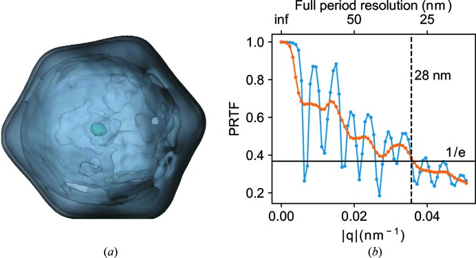
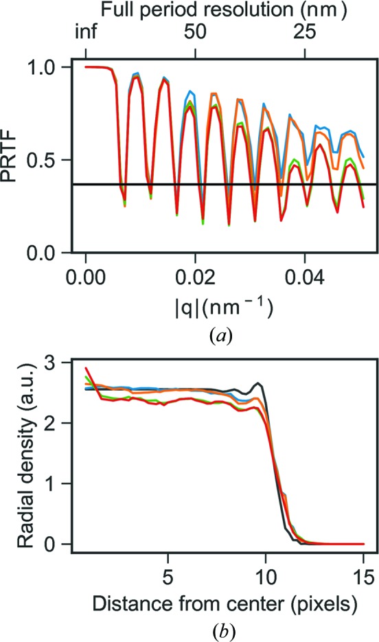
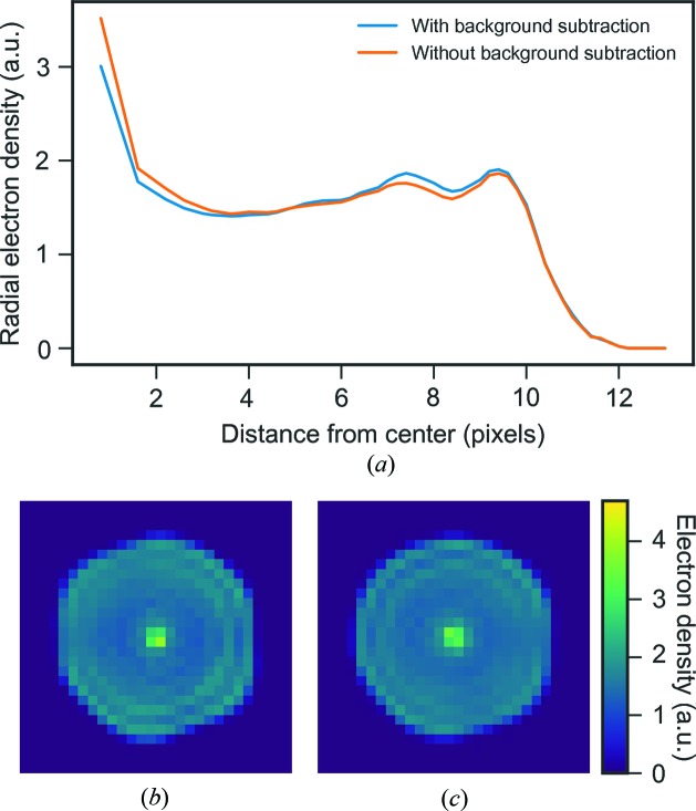
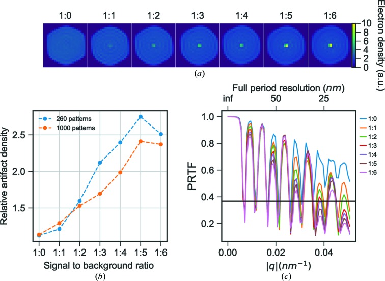
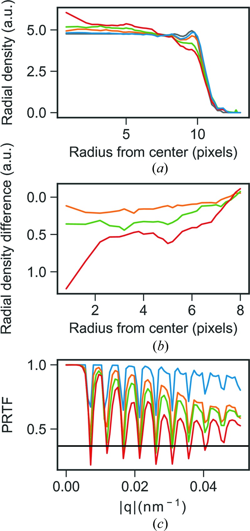
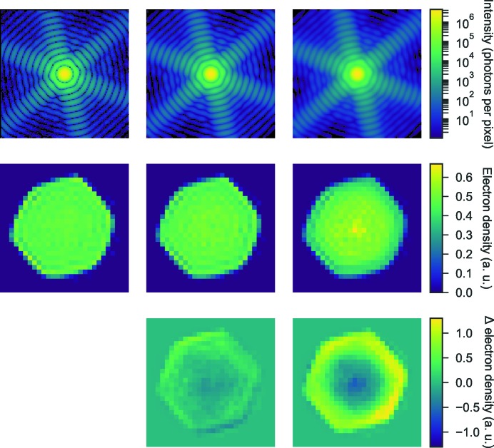
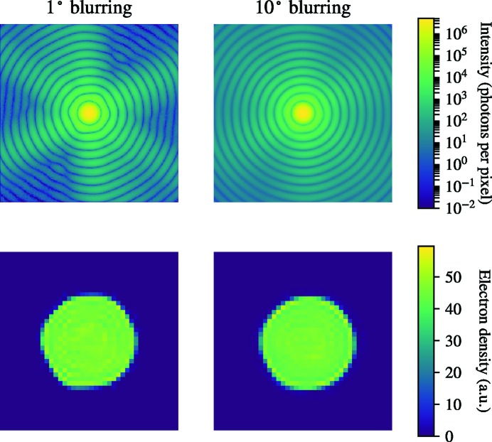
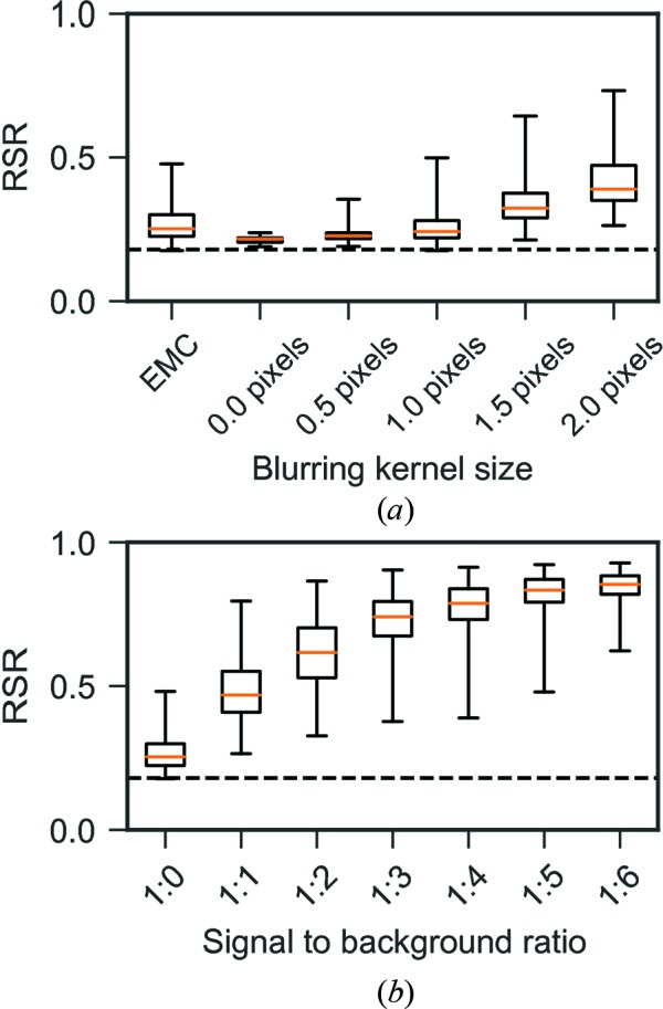
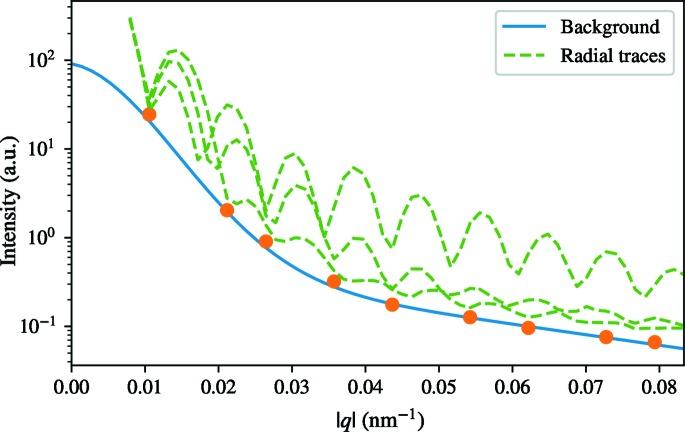
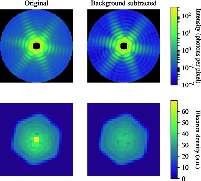
Diffraction before destruction using X-ray free-electron lasers (XFELs) has the potential to determine radiation-damage-free structures without the need for crystallization. This article presents the three-dimensional reconstruction of the Melbournevirus from single-particle X-ray diffraction patterns collected at the LINAC Coherent Light Source (LCLS) as well as reconstructions from simulated data exploring the consequences of different kinds of experimental sources of noise. The reconstruction from experimental data suffers from a strong artifact in the center of the particle. This could be reproduced with simulated data by adding experimental background to the diffraction patterns. In those simulations, the relative density of the artifact increases linearly with background strength. This suggests that the artifact originates from the Fourier transform of the relatively flat background, concentrating all power in a central feature of limited extent. We support these findings by significantly reducing the artifact through background removal before the phase-retrieval step. Large amounts of blurring in the diffraction patterns were also found to introduce diffuse artifacts, which could easily be mistaken as biologically relevant features. Other sources of noise such as sample heterogeneity and variation of pulse energy did not significantly degrade the quality of the reconstructions. Larger data volumes, made possible by the recent inauguration of high repetition-rate XFELs, allow for increased signal-to-background ratio and provide a way to minimize these artifacts. The anticipated development of three-dimensional Fourier-volume-assembly algorithms which are background aware is an alternative and complementary solution, which maximizes the use of data.

Keywords: LCLS; Melbournevirus; XFELs; coherent diffractive imaging; image reconstruction.

Figure 1

Lit-pixel threshold determination for a typical recorded run. The first 287 patterns from the run were manually classified into hits and misses. Those patterns were then sorted, by the number of lit pixels, into 20 bins. The hit fraction for each bin is shown along with a fitted Gauss-error function. The point at which the fit reaches a hit fraction of 0.5 determines the lit-pixel threshold used for automatic hit finding in the Cheetah software package (Barty et al., 2014 ▸).

Figure 2

Nine high-quality diffraction patterns of MelV from the experiment. Gray areas represent masked-out regions.

Figure 3

(a) Slices from three-dimensional reconstructions from three different image selections: a manual selection of 670 patterns from a 2 h data collection (blue), an automatic image selection of 586 patterns with a subsequent manual sub-selection (orange) and a tighter size restriction on the orange image selection consisting of 260 patterns (green). (b) Radial average plots of the reconstructions and (c) their corresponding PRTF. The colors represent the same image selection in all three sub-figures.

Figure 4

Histograms of MelV sizes retrieved through sphere fit on experimental data, comparing different image selections. Manual selection from one run (blue), automatic image selection with manual clean up (orange) and sub-selection with narrow size distribution (green). The color coding for the image selections is the same as in Fig. 3 ▸. The dashed lines in all histograms represent the median size of the distribution.

Figure 5

(a) Three-dimensional representation of the reconstruction from experimental data (a strict selection of 260 patterns with a limited size distribution). (b) PRTF for the reconstruction in (a). The blue line represents the radial average of the three-dimensional PRTF and the orange line is the critically sampled three-dimensional PRTF. The critically sampled PRTF shows a full-period resolution of 28 nm.

Figure 6

(a) PRTF and (b) radial average for three-dimensional reconstructions from homogeneous simulated data (blue), heterogeneous data (orange), homogeneous data with background (green) and heterogeneous data with background (red). The black curve represents the radial average of the input model scaled according to central density of the reconstruction from homogeneous data without added background.

Figure 7

(a) Radial average of three-dimensional reconstructions for experimental data with (blue) and without (orange) background subtraction applied on the raw images. The images show slices through the three-dimensional reconstructions with background subtraction applied to the raw images (b) and without background subtraction (c).

Figure 8

(a) Slices through reconstructions from simulated data with experimental background added in increasing proportions (ratio indicated above each image). (b) The calculated relative density of the 8 voxel central artifact compared with the median density of the particle interior for reconstructions with increasing proportion of experimental background from simulated data using 1000 (orange) and 260 (blue) images. (c) The PRTF for the reconstructions.

Figure 9

(a) Radial averages of reconstructions from blurred models with Gaussian blur kernels of 0 (blue), 1.0 (orange), 1.5 (green) and 2.0 (red). In gray is the radial average of the input model used in the simulations scaled to the reconstructed models. (b) Differences in radial averages from left plot, blur1.0 − blur0 (orange), blur1.5 − blur0 (green) and blur2.0 − blur0 (red). (c) PRTF for the reconstructions from blurred models with Gaussian blur kernels of 0 (blue), 1.0 (orange), 1.5 (green) and 2.0 (red).

Figure 10

Reconstructions from blurred three-dimensional Fourier volumes. The first row of images shows one slice through the 8 times downsampled Fourier volumes in log scale with no blur (left), 1-pixel standard deviation Gaussian blur (middle) and 2-pixel standard deviation Gaussian blur (left). The second row shows slices through the corresponding three-dimensional reconstructions. The last row of images shows the difference in density between the reconstruction from the non-blurred and blurred Fourier volumes, with 1-pixel (left) and 2-pixel (right) standard deviation of the Gaussian blurring kernels.

Figure 11

The intensity space was rotationally blurred with a standard deviation of 1 and 10°. Slices through the resulting Fourier intensities (top) are shown together with the corresponding reconstructed electron densities (bottom). This type of blurring did not produce the same type of artifacts as we saw when the blur also included the radial direction.

Figure 12

(a) RSR box and whisker plots for reconstructions from three-dimensional Fourier volumes blurred with a Gaussian kernel of increasing width. RSR for a model from simulated two-dimensional patterns oriented with EMC is shown as a comparison to the blurred models. (b) RSR box and whisker plot for reconstructions with increasing background ratio. The dashed horizontal line shows the RSR for the input model in both box plots. The mean RSR is shown with an orange line, the boxes indicate the interquartile range and the whiskers represent the lowest and highest RSR value for each group.

Figure 13

The blue line shows the radial background that was subtracted from the Fourier intensities before phase retrieval. The function is a fit to the orange points which represents the lowest points in the radial minimum function. The green lines show the values among three radial lines from the center of the Fourier intensities. As expected the background is below the signal levels at all points.

Figure 14

The top row shows a slice through the Fourier intensities after EMC. The left panel shows the untreated output from EMC while the right panel shows the result of the background subtraction. The background-subtracted version shows more well defined minima and clearer streaks. The bottom row shows the corresponding reconstructions. The reconstruction of the background subtracted version is very similar except that it is almost free from the strong artifact in the center that plagued the original reconstruction.

References

1. Altarelli, M. et al. (2007). The European X-ray Free-Electron Laser. Technical Design Report 2006-097. DESY, Hamburg, Germany.
1. Barty, A., Kirian, R. A., Maia, F. R. N. C., Hantke, M., Yoon, C. H., White, T. A. & Chapman, H. (2014). J. Appl. Cryst. 47, 1118–1131. - PMC - PubMed
1. Bergh, M., Huldt, G., Tîmneanu, N., Maia, F. R. N. C. & Hajdu, J. (2008). Q. Rev. Biophys. 41, 181–204. - PubMed
1. Bozek, J. D. (2009). Eur. Phys. J. Spec. Top. 169, 129–132.
1. Chapman, H. N., Barty, A., Bogan, M. J. et al. (2006). Nat. Phys. 2, 839–843.