Transition state characteristics during cell differentiation

Abstract

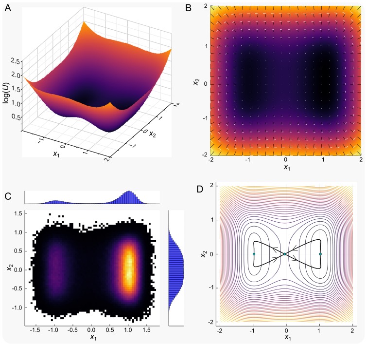
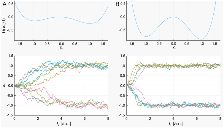
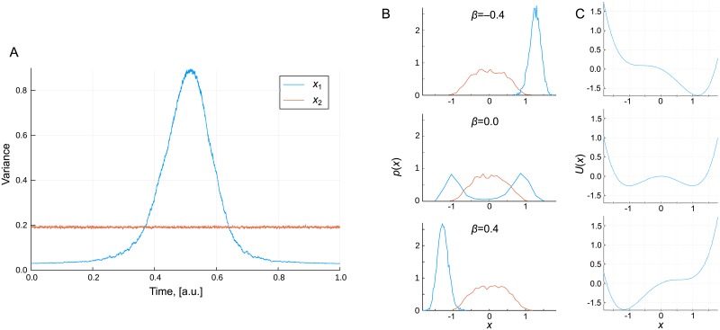
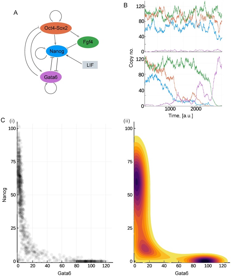
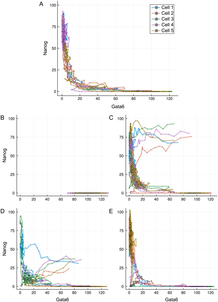
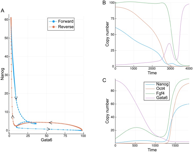
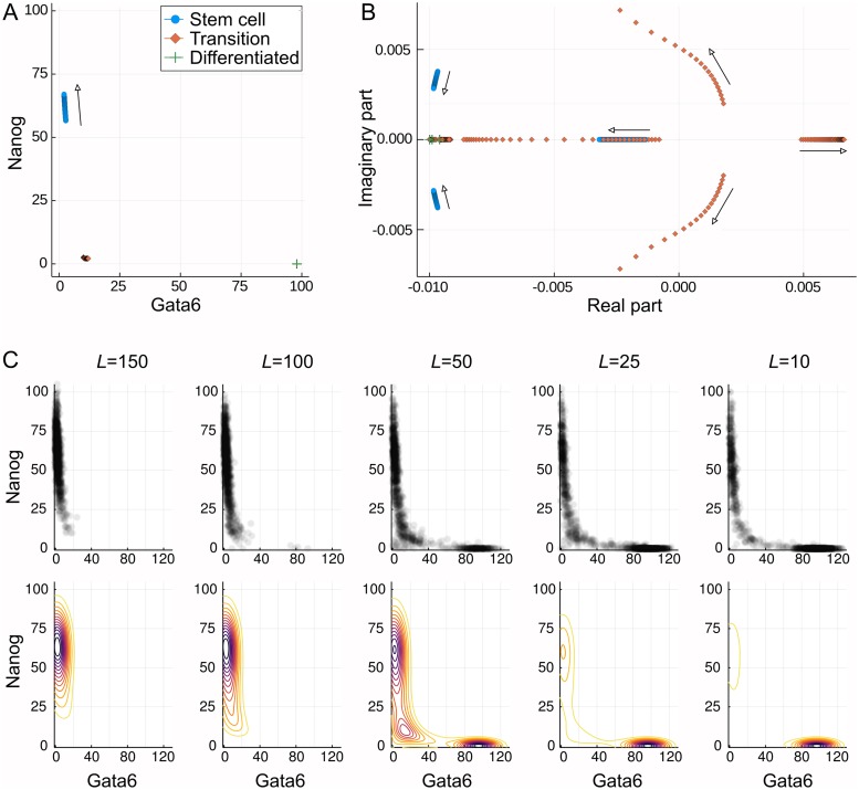
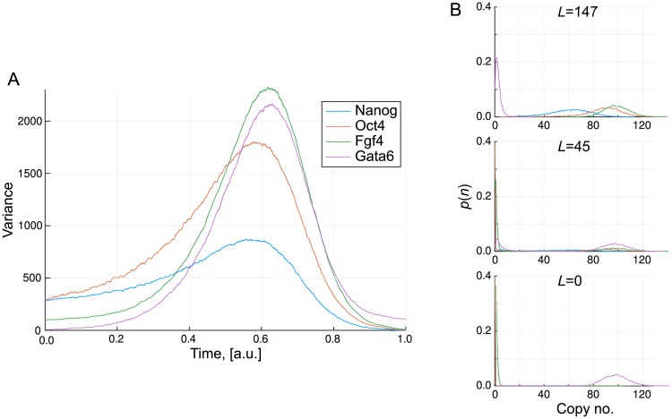
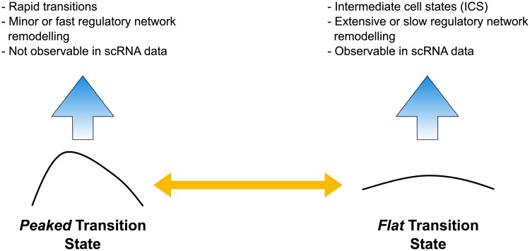
Models describing the process of stem-cell differentiation are plentiful, and may offer insights into the underlying mechanisms and experimentally observed behaviour. Waddington's epigenetic landscape has been providing a conceptual framework for differentiation processes since its inception. It also allows, however, for detailed mathematical and quantitative analyses, as the landscape can, at least in principle, be related to mathematical models of dynamical systems. Here we focus on a set of dynamical systems features that are intimately linked to cell differentiation, by considering exemplar dynamical models that capture important aspects of stem cell differentiation dynamics. These models allow us to map the paths that cells take through gene expression space as they move from one fate to another, e.g. from a stem-cell to a more specialized cell type. Our analysis highlights the role of the transition state (TS) that separates distinct cell fates, and how the nature of the TS changes as the underlying landscape changes-change that can be induced by e.g. cellular signaling. We demonstrate that models for stem cell differentiation may be interpreted in terms of either a static or transitory landscape. For the static case the TS represents a particular transcriptional profile that all cells approach during differentiation. Alternatively, the TS may refer to the commonly observed period of heterogeneity as cells undergo stochastic transitions.

Fig 1. The two-dimensional SDE model.

(A) surface plot of the potential field U; (B) the vector field decomposed into the gradient (black) and curl (white) components; (C) the two-dimensional histogram generated from a long-run simulation of the system; (D) The minimum action paths (MAP) between stationary points X_i. On exit from an attractor the MAP follows a path $\dot{X}=\nabla U+f_U$, before following a “free fall” path back towards a stationary point.

Fig 2. Influence of eigenvalues.

Slice through the potential and example trajectories away from the transition state under different model parameters: (A) small positive eigenvalue (α = 0.4); (B) large positive eigenvalue (α = 1.6). For a larger positive eigenvalue the wells of the system are deeper and the curvature is greater, leading to more rapid movement away from the transition state.

Fig 3. The transition state in a transitory landscape.

(A) The variance of the two states across 5000 simulations in which β is linearly varied with time; (B) Probability distributions of the two states at three different values of β; (C) The potential U at each of the three values of β. The high variance “transition state” corresponds to intermediate values of β in which significant bistability generates large heterogeneity.

Fig 4. Potential landscape of the stem cell differentiation model.

(A) Schematics of the stem cell differentiation model. (B) Simulated example of a cell that stays pluripotent (upper axes) and a cell undergoing differentiation (lower axes). The abundance of each species is indicated by a line coloured according to the filled ovals in (A). (C) Probability distribution and landscape of the system with L = 50. (i) Scatter plot of the whole population on the Gata6-Nanog plane. (ii) The landscape computed as the negative logarithm of the probability distribution.

Fig 5. Transition paths during differentiation.

(A) Trajectories of five randomly selected stem cells after reduction in LIF concentration (L = 0), plotted on the Gata6-Nanog phase space. (B) Cells started from the differentiated state and put into L = 200. (C-D) Cells started from the unexplored region of high Gata6 and high Nanog (C) or low Nanog (D) levels for L = 0. (E) Trajectories started from the transition state under L = 50. Different line colours denote different cells, as indicated in the legend.

Fig 6. Minimum action paths for the developmental model.

(A) A comparison of the paths plotted in the Gata6, Nanog plane; (B) Time series for each of the molecular species in the forward direction; (C) Time series for each of the molecular species in the reverse direction.

Fig 7. Varying behaviour of the system with LIF concentration, L.

(A) Three of the fixed points of the model with increasing L. The differentiated and transition state remain unchanged while the stem cell state moves to higher Nanog values. (B) The eigenvalues of the Jacobian at each of the three fixed points as L increases. The stem cell state becomes locally more stable, as indicated by the increasingly negative eigenvalues. The transition state becomes increasingly unstable, thereby making transition to this state less probable. The differentiated state is unaffected, but is seen to be locally more stable than the stem cell state. Complex eigenvalues are associated with rotational “curl” dynamics. (C) Variation of the probabilistic landscape. Upper plots show a sample of the sampled points while lower plots show the landscapes. As L decreases the valley at the differentiated state becomes deeper while that at the stem cell state becomes shallower. At intermediate values the landscape is flatter around the transition state.

Fig 8. The transition state in a transitory landscape.

(A) The variance of the transcription levels across 10,000 simulations in which L is linearly decreased with time as L = 150(1 − t); (B) Probability distributions of the transcription levels at three different values of L. The high variance “transition state” corresponds to intermediate values of L at which transitions from the stem cell to differentiated state begin to occur.

Fig 9. Relationship between transition state and observable data.

The landscape curvature around the TS affects the time cells will spend in the vicinity of the TS, and reflects the molecular processes driving differentiation.

References

1. Waddington CH. The strategy of the genes: a discussion of some aspects of theoretical biology. London: Allen & Unwin; 1957.
1. Filippi S, Barnes CP, Kirk PDW, Kudo T, Kunida K, McMahon SS, et al. Robustness of MEK-ERK Dynamics and Origins of Cell-to-Cell Variability in MAPK Signaling. Cell Reports. 2016;15(11):2524–2535. 10.1016/j.celrep.2016.05.024 - DOI - PMC - PubMed
1. Hormoz S, Singer ZS, Linton JM, Antebi YE, Shraiman BI, Elowitz MB. Inferring Cell-State Transition Dynamics from Lineage Trees and Endpoint Single-Cell Measurements. Cell Systems. 2016;3(5):419–433.e8. 10.1016/j.cels.2016.10.015 - DOI - PMC - PubMed
1. Moris N, Martinez-Arias A. The Hidden Memory of Differentiating Cells. Cell Systems. 2017;5(3):163–164. 10.1016/j.cels.2017.09.009 - DOI - PubMed
1. Moris N, Pina C, Arias AM. Transition states and cell fate decisions in epigenetic landscapes. Nature Reviews Genetics. 2016;(11):693–703. 10.1038/nrg.2016.98 - DOI - PubMed
Publication types