. 2018 Sep 26:7:e37349.
doi: 10.7554/eLife.37349.

Sparse recurrent excitatory connectivity in the microcircuit of the adult mouse and human cortex

Affiliations

Sparse recurrent excitatory connectivity in the microcircuit of the adult mouse and human cortex

Stephanie C Seeman et al. Elife. .

Abstract

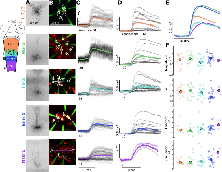
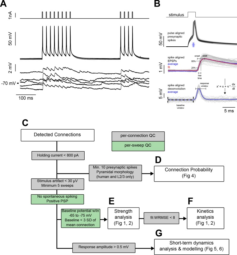
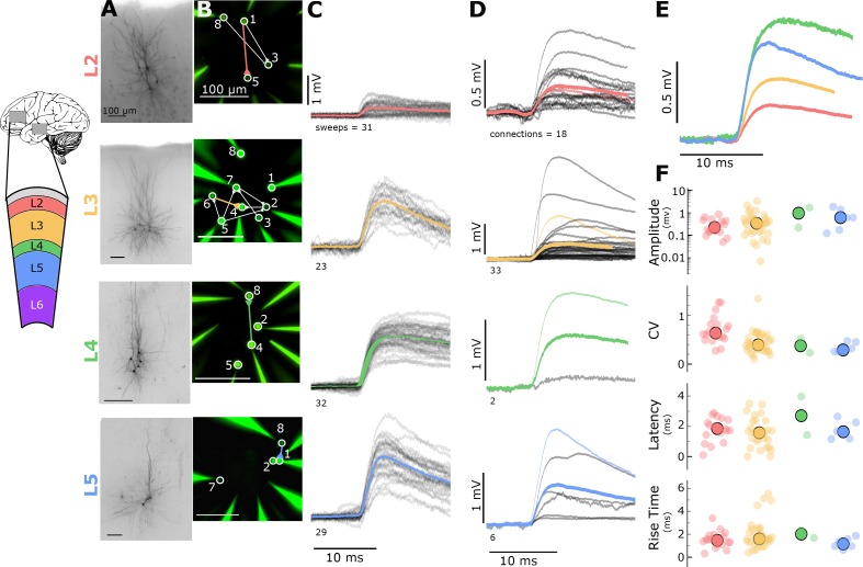
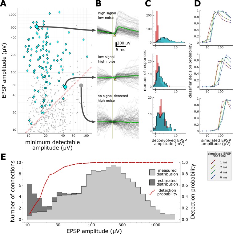
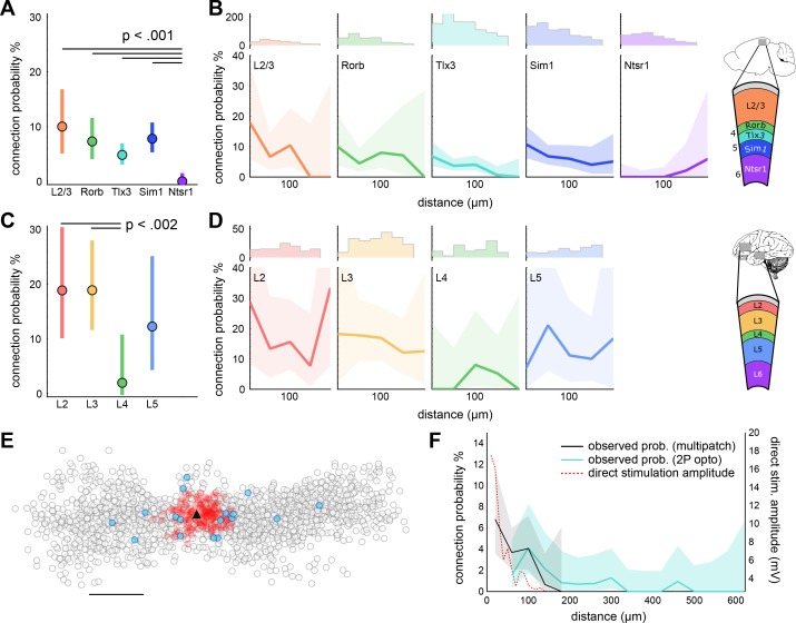
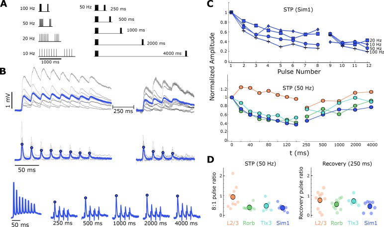
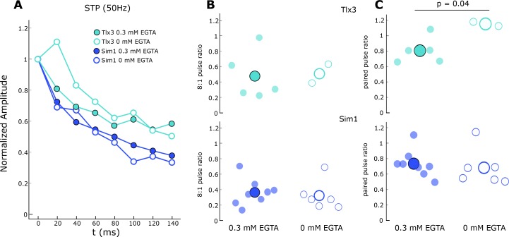
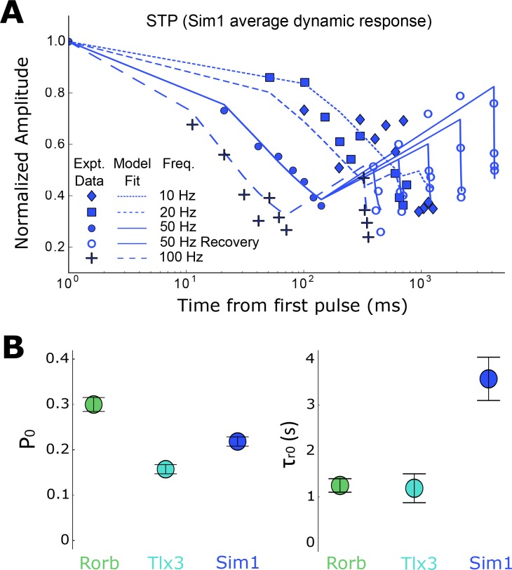
Generating a comprehensive description of cortical networks requires a large-scale, systematic approach. To that end, we have begun a pipeline project using multipatch electrophysiology, supplemented with two-photon optogenetics, to characterize connectivity and synaptic signaling between classes of neurons in adult mouse primary visual cortex (V1) and human cortex. We focus on producing results detailed enough for the generation of computational models and enabling comparison with future studies. Here, we report our examination of intralaminar connectivity within each of several classes of excitatory neurons. We find that connections are sparse but present among all excitatory cell classes and layers we sampled, and that most mouse synapses exhibited short-term depression with similar dynamics. Synaptic signaling between a subset of layer 2/3 neurons, however, exhibited facilitation. These results contribute to a body of evidence describing recurrent excitatory connectivity as a conserved feature of cortical microcircuits.

Keywords: cortical wiring; electrophysiology; human; mouse; neuroscience; short term plasticity.


Conflict of interest statement

SS, LC, PD, AH, TH, AB, CB, JL, SM, CT, AK, JO, RG, DS, CC, JP, EL, GM, CK, HZ, TJ No competing interests declared

Figures

Figure 1.
Figure 1.. Electrophysiological recordings of evoked excitatory synaptic responses between individual cortical pyramidal neurons in mouse primary visual cortex.
(A) Cartoon illustrating color, Cre-line, and cortical layer mapping in slice recording region (V1). Example maximum intensity projection images of biocytin-filled pyramidal neurons for L2/3 and each Cre line. (B) Example epifluorescent images of neurons showing Cre-dependent reporter expression and/or dye-filled recording pipettes. Connection map is overlaid on the epifluorescent image (colored: example connection shown in C). (C) Spike time aligned EPSPs induced by the first AP of all ≤ 50 Hz stimulus trains for a single example connection (individual pulse-response trials: grey; average: colored). (D) First pulse average, like in C., for all connections within the synaptic type; grey: individual connections; thin-colored: connection highlighted in C; thick-colored: grand average of all connections. (E) Overlay of grand average for each connection type. (F) EPSP amplitude (in log units), CV of amplitude, latency, and rise time of first-pulse responses for each Cre-type (small circles) with the grand median (large). See Figure 1—figure supplement 1 for data processing and analysis diagrams.
Figure 1—figure supplement 1.
Figure 1—figure supplement 1.. Experiment methodology and analysis workflow.
(A) Example connected pair showing the stimulation pulses (top) and action potentials (middle) in the presynaptic cell; monosynaptically evoked EPSPs (bottom) in the postsynaptic cell. Traces represent every fifth sweep from the 50 Hz protocol used to measure recovery from STP at a delay of 250 ms. (B) Following repeated stimulation, the response to the first spike in each train of current pulsess was used for EPSP feature analysis. Spikes are shown aligned to the pulse time to illustrate jitter in spike timing. Spike time was defined as the region of maximum dV/dt in the spike trace, as shown in the raster plot corresponding to spike timing of individual spikes. Below, EPSPs are aligned to the spike time prior to fitting the average EPSP (see Equation 1; individual sweeps in grey, average response in blue, fit shown in red). The rise time was calculated as the interval between 20% and 80% of the peak amplitude of the fit. Spike-aligned EPSPs were deconvolved (see Equation 2, shown in figure), and the peak amplitudes of the deconvolved traces were used to measure changes in response amplitude of the course of a spike train. Responses were corrected to the baseline by subtracting the mode of the region between 10 ms and 50 µs prior to stimulus onset (baseline window). Responses were measured as the peak response during a 4 ms window beginning 1 ms after the spike time (response window shown is aligned to mean spike time). (C–G) Subsets of total connectivity data were used in subsequent analysis. Flowchart shows sweep (green) and connection (grey) level inclusion criteria for data included in each figure. See Table 1 for total number of cells in each criterion.
Figure 2.
Figure 2.. Electrophysiological recordings of evoked excitatory synaptic responses between individual human cortical pyramidal neurons.
(A) Cartoon illustrating color and cortical layer mapping in slice recording region (temporal or frontal cortex). Example maximum intensity projection images of biocytin-filled pyramidal neurons for layers 2–5. (B) Example epifluorescent images of neurons showing dye-filled neurons and recording pipettes. Connection map is overlaid on the epifluorescent image (colored: example connection shown in C). (C) Spike time aligned EPSPs induced by the first AP of all ≤ 50 Hz stimulus trains for a single example connection (individual pulse-response trials: grey; average: colored). (D) First pulse average, like in C., for all connections within the synaptic type; grey: individual connections; thin-colored: connection highlighted in C; thick-colored: grand average of all connections. (E) Overlay of grand average for each connection type. (F) EPSP amplitude, CV of amplitude, latency, and rise time of first-pulse responses for each layer (small circles) with the grand mean (large circles). See Figure 1—figure supplement 1 for data processing and analysis diagrams.
Figure 3.
Figure 3.. Characterization of synapse detection limits.
(A) Scatter plot showing measured EPSP amplitude versus minimum detectable amplitude for each tested pair. Detected synapses (manually annotated) are shown as blue diamonds; pairs with no detected EPSPs are grey dots. The region under the red dashed line denotes the region in which synaptic connections are likely to be misclassified as unconnected. Three example putative connections are highlighted in A and described further in panels B-D. One connection (top row) was selected for its large amplitude PSP and low background noise. Another connection (middle row) is harder to detect (PSP onset marked by yellow arrowhead) due to low amplitude and high background noise. The bottom row shows a recorded pair that was classified as unconnected. (B) A selection of postsynaptic current clamp recordings in response to presynaptic spikes. Each row contains recordings from a single tested pair. The vertical line indicates the time of presynaptic spikes, measured as the point of maximum dV/dt in the presynaptic recording. Yellow triangles indicate the onset of the EPSP. (C) Histograms showing distributions of peak response values measured from deconvolved traces (see Materials and methods). Red area indicates measurements made on background noise; blue area indicates measurements made immediately following a presynaptic spike. (D) Characterization of detection limits for each example. Plots show the probability that simulated EPSPs would be detected by a classifier, as a function of the rise time and mean amplitude of the EPSPs. Each example has a different characteristic detection limit that depends on the recording background noise and the length of the experiment. (E) An estimate of the total number of false negatives across the entire dataset. The measured distribution of EPSP amplitudes is shown in light grey (smoothed with a Gaussian filter with σ = 1 bin). The estimated correction show in dark grey is derived by dividing the measured distribution by the overall probability of detecting a synapse (red dashed line) at each amplitude. See Supplementary file 1 for features included in classifier.
Figure 4.
Figure 4.. Distance dependent connectivity profiles of mouse and human E-E connections.
(A) Recurrent connection probability and distribution of connections for mouse -linesand layer 2/3. Mean connection probability (filled circles) and 95% confidence intervals (bars) for connections probed within 100 µm (n connections in Table 1). (B) Connection probability over distance for mouse Cre-lines and layer 2/3. Top: Histogram of putative connections probed. Bottom: Mean connection probability (thick line) with 95% confidence intervals (shading) binned in 40 µm increments. (C) Like-to-like connection probability and distribution of connections between human pyramidal neurons. Mean connection probability (filled circles) and 95% confidence intervals (bars) for connections probed within 100 µm. (D) Connection probability over distance for human pyramidal neurons, formatted as in panel B. (E) Tlx3-Tlx3 connection probability measured by two-photon mapping. X-Y distance distribution of connections probed onto a postsynaptic cell (black triangle), detected presynaptic neurons (filled circles), no connection detected (empty circles), and direct event artifact due to undesired activation of opsin in the dendritic arbor of the recorded cell (red circles). (F) Connection probability and stimulation artifact over distance measured by two-photon mapping. Mean connection probability vs. distance (blue line; starting at 50 µm) with 95% confidence intervals (shading) and direct event artifact amplitude vs. distance (dotted red line) for Tlx3-Tlx3 connections probed with two-photon stimulation. See Figure 4—figure supplement 3 for distribution of connectivity as a function of cortical slice position and cell depth. See Figure 4—figure supplements 1,2 for details on two-photon connectivity experiments.
Figure 4—figure supplement 1.
Figure 4—figure supplement 1.. Intralaminar connectivity rates were unaffected by recording depth and medial-lateral position in V1.
(A) Connectivity rate was assessed as a function of slice number, spanning a total sampled region across experiments of 3.5 mm of cortex (350 µm per slice). (B) The observed synaptic connectivity (open circles) and 95% CI (grey region) are shown relative to overall average connectivity (dotted line). (C) Connectivity was not influenced by depth from the slice surface between −40 and −200 µm. Sampling frequency and connectivity as a function of depth from slice surface are shown in D.
Figure 4—figure supplement 2.
Figure 4—figure supplement 2.. Characterization of two-photon photostimulation.
(A) Cartoon illustrating loose-seal recording configuration utilized to test photostimulation parameters. Example recording of repeated photostimulation or a ReaChR-positive cell. (B) Cumulative probability plot of minimum power necessary to reliably evoke action potentials for 13 cells. Blue dashed lines indicate light power utilized in mapping experiments and the fraction of cells reliably activated. (C) Average latency of light-evoked action potentials plotted against photostimulation intensity for individual neurons (grey dashed lines). Filled black circle and error bars represent the mean and standard deviation of latency measured across all cells at a power used for mapping. (D) Average jitter of light-evoked action potentials plotted against photostimulation intensity. Data from individual cells and population average plotted as in panel C. (E) Left: Example experiment illustrating the radial grid pattern used to measure the lateral resolution of photostimulation and example traces recorded during the photostimulation at indicated locations. Right: Probability of generating light-evoked action potentials plotted against lateral distance from the center of the cell. (F) Left: example of responses resulting from photostimulation at indicated axial offsets. Right: Probability of generating light-evoked action potentials plotted against axial distance from the center of the cell.
Figure 4—figure supplement 3.
Figure 4—figure supplement 3.. Two-photon optogenetic mapping details.
(A) Maximum intensity projection of Tlx3-Cre:Ai136 slice and a recorded neuron. Blue circle denotes location of stimulated presynaptic neuron. (B) Top: Electrophysiological recording of postsynaptic response to 10 photostimulations of the presynaptic neuron in panel A. Timing of photostimulation indicated by pink shading. Synaptic events detected by exponential deconvolution are indicated by inverted triangles. Events used to produce average synaptic response are show in blue. Bottom: Peri-stimulus event histogram. (C) Individual events aligned by the timing of event detection (grey) and average EPSP (blue). (D) Signal versus noise plot for all optogenetically-probed presynaptic neurons. (E) Cumulative probability plot of signal-to-noise ratios for stimulus trials scored as no connection, connection, or containing a direct stimulation artifact. Dashed grey line indicates signal-to-noise ratio = 1.
Figure 5.
Figure 5.. Short-term dynamics of mouse recurrent connections by Cre-line and layer (n in Table 1 ‘STP’).
(A) Schematic of STP and STP recovery stimuli. (B) Sim1-Cre EPSPs in response to a 50 Hz stimulus train (top; eight induction pulses and four recovery pulses delayed 250 ms; individual connection: gray traces; blue: Sim1-Cre average EPSP at 50 Hz). Exponential deconvolution followed by lowpass filter of EPSPs above (middle, filled circles: pulse amplitudes in C). Exponential deconvolution of 50 Hz stimulus with all five recovery time points in A (bottom, filled circles: pulse amplitudes in C). (C) The mean normalized amplitude of deconvolved response versus pulse number at multiple stimulation frequencies for Sim1-Cre (top). Normalized amplitude of the deconvolved response at 50 Hz with first recovery pulse at each interval for each Cre-line and L2/3 connections (bottom). (D) The depth of depression during 50 Hz induction (left) as measured by the amplitude ratio of the 8th to 1st pulse for each Cre-line and layer (small circles) and grand mean (large circles). Amount of recovery at 250 ms latency (right) for each Cre-line and layer (small circles) and grand mean (large circles). See Figure 5—figure supplement 1 for results of STP at different EGTA concentrations and Figure 1—figure supplement 1 for data analysis diagram.
Figure 5—figure supplement 1.
Figure 5—figure supplement 1.. Influence of internal EGTA on short-term dynamics.
(A) Normalized response amplitude during a 50 Hz train in Tlx3 (cyan) and Sim1 (blue) connections with 0.3 mM EGTA present in the internal solution (filled) and in the absence of EGTA (open). Data are grand average of all connections within each type. (B) Ratio of the last (8th) pulse in the train to the first for each connection within each type (small circles) and the grand mean (large circle); colors and fill follow as in A. (C) Paired-pulse ratio for each connection within each type (small circles) and the grand mean (large circles); colors and fill follow as in A.
Figure 6.
Figure 6.. Modeling of short-term depression in recurrent Rorb, Sim1, and Tlx3 connections (n in Table 1 ‘STP’).
(A) Sim1 average dynamic response; Same data as in Figure 5C, top plotted on a log-X time scale with modeling fits overlaid. (B) Results of model for parameters P0 and 𝜏r0. Values are means with standard error of the covariance matrix. Paired Z-scores (Equation 6) in Table 5.

Similar articles

Cited by

References

    1. Abbott LF, Varela JA, Sen K, Nelson SB, Sen N. Synaptic depression and cortical gain control. Science. 1997;275:221–224. doi: 10.1126/science.275.5297.221. - DOI - PubMed
    1. Barth L, Burkhalter A, Callaway EM, Connors BW, Cauli B, DeFelipe J, Feldmeyer D, Freund T, Kawaguchi Y, Kisvarday Z, Kubota Y, McBain C, Oberlaender M, Rossier J, Rudy B, Staiger JF, Somogyi P, Tamas G, Yuste R. Comment on "Principles of connectivity among morphologically defined cell types in adult neocortex". Science. 2016;353:1108. doi: 10.1126/science.aaf5663. - DOI - PubMed
    1. Biane JS, Scanziani M, Tuszynski MH, Conner JM. Motor cortex maturation is associated with reductions in recurrent connectivity among functional subpopulations and increases in intrinsic excitability. Journal of Neuroscience. 2015;35:4719–4728. doi: 10.1523/JNEUROSCI.2792-14.2015. - DOI - PMC - PubMed
    1. Binzegger T, Douglas RJ, Martin KA. A quantitative map of the circuit of cat primary visual cortex. Journal of Neuroscience. 2004;24:8441–8453. doi: 10.1523/JNEUROSCI.1400-04.2004. - DOI - PMC - PubMed
    1. Bopp R, Maçarico da Costa N, Kampa BM, Martin KA, Roth MM, Kampa, KAC M R. Pyramidal cells make specific connections onto smooth (GABAergic) neurons in mouse visual cortex. PLoS Biology. 2014;12:e1001932. doi: 10.1371/journal.pbio.1001932. - DOI - PMC - PubMed

Publication types

LinkOut - more resources