A MATLAB toolbox for multivariate analysis of brain networks

Abstract

Complex brain networks formed via structural and functional interactions among brain regions are believed to underlie information processing and cognitive function. A growing number of studies indicate that altered brain network topology is associated with physiological, behavioral, and cognitive abnormalities. Graph theory is showing promise as a method for evaluating and explaining brain networks. However, multivariate frameworks that provide statistical inferences about how such networks relate to covariates of interest, such as disease phenotypes, in different study populations are yet to be developed. We have developed a freely available MATLAB toolbox with a graphical user interface that bridges this important gap between brain network analyses and statistical inference. The modeling framework implemented in this toolbox utilizes a mixed-effects multivariate regression framework that allows assessing brain network differences between study populations as well as assessing the effects of covariates of interest such as age, disease phenotype, and risk factors on the density and strength of brain connections in global (i.e., whole-brain) and local (i.e., subnetworks) brain networks. Confounding variables, such as sex, are controlled for through the implemented framework. A variety of neuroimaging data such as fMRI, EEG, and DTI can be analyzed with this toolbox, which makes it useful for a wide range of studies examining the structure and function of brain networks. The toolbox uses SAS, R, or Python (depending on software availability) to perform the statistical modeling. We also provide a clustering-based data reduction method that helps with model convergence and substantially reduces modeling time for large data sets.

Keywords: MATLAB toolbox; brain connections; brain networks; mixed-effects regression; multivariate modeling.

Figure 1

The framework of the WFU_MMNET. Both ROI time series and connection matrices obtained from preprocessed data from different neuroimaging modalities (e.g., fMRI, EEG, or MEG) can be used in WFU_MMNET. Connection matrices obtained from computing associations between time series in functional brain data or white matter tracks in structural data are depicted with colored squares in this cartoon figure. Exogenous variables including the covariate of interest (e.g., a binary variable distinguishing study populations or a continuous variable if individual differences are of interest), disease phenotypes (e.g., phenotypes measured via blood samples or imaging modalities), risk factors (e.g., hypertension or smoking), and other covariates of interest such as age can be loaded into the toolbox as a matrix. WFU_MMNET provides quantified relationships between brain (structural or functional) connections as the outcome variable and topological brain network features and exogenous variables. Significant differences of brain network topologies or features between study populations as well as different impacts of exogenous variables on the (density and strength of) brain connections between study populations can be obtained via interaction variables (i.e., interactions of the variable distinguishing study populations and network covariates or any other desired covariate) [Color figure can be viewed at http://wileyonlinelibrary.com]

Figure 2

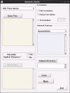
WFU_MMNET main (starting) graphical user interface. This GUI can be started by running the “WFU_MMNET.m” function or typing “WFU_MMNET” in the command window of MATLAB. Modeling is done in two main steps. In the first step, using imaging data files (and atlas files), initial modeling files, such as an initial data frame, are generated through the “Network_Model” GUI. This step is independent of the second step and can be repeated for different imaging data or different options on the same data set. In the second step, using generated files from the first step, final modeling files, including modeling data sets, equations, and options are generated, and the statistical models are fitted. The second step is done through the “Statistical_Model” GUI. This step can also be done repeatedly for different options as long as an initial modeling file is available [Color figure can be viewed at http://wileyonlinelibrary.com]

Figure 3

The network model GUI. This GUI can be started by clicking the “Network Model” button on the “WFU_MMNET” GUI (Figure 2). After loading required files and selecting desired options, initial modeling files will be generated and saved in the output directory. These files will later be used in the second step to generate final modeling files and fit statistical models [Color figure can be viewed at http://wileyonlinelibrary.com]

Figure 4

The statistical model GUI. This GUI can be started by clicking the “Statistical Model” button on the “WFU_MMNET” GUI (Figure 2). Generated modeling files from the first step will be used here to make the final modeling data sets, equations, and options, and fit the statistical models. Modeling is conducted automatically via a system call of the SAS, R, or Python executable files. The user should add the modeling software prior to starting the toolbox as detailed in the manual [Color figure can be viewed at http://wileyonlinelibrary.com]

Figure 5

Diagram of the modeling approach. The ROI time series is used to compute the connection matrix with negative values set to zero. Each region of the brain serves as a network node. The binarized connection matrix is obtained by setting all nonzero values of the connection matrix to one. The network measures extracted from the connection matrix along with exogenous variables of interest, the interaction variables, and confounding variables will be used as covariates in the two‐part mixed‐effects modeling framework. The brain network shown in this figure was generated (for illustrative purposes only) using BrainNet Viewer toolbox [Xia et al., 2013]) [Color figure can be viewed at http://wileyonlinelibrary.com]

Figure 6

Clustering‐based data size reduction method implemented in WFU_MMNET. To ensure the same percentage of data samples is preserved for each participant, the clustering is applied on each participant's data samples separately instead of clustering the final data set which contains data samples of all participants. Number of clusters in this method is determined by the percentage of the data that is selected to be removed (e.g., if 80% (0.8) of data samples should be discarded and a participant has 6,000 samples, this participant's data will be split into 1,200 clusters ([100–80] × 0.1 × 6,000)). Since the same percentage of data samples are removed for each participant, the final data set also has the same percentage of its original size removed. Data samples of each participant are clustered using a k‐means clustering (implemented in MATLAB) method, then the samples closest to the center of each cluster are preserved while discarding other ones. This process is repeated for all participants yielding the final reduced data set [Color figure can be viewed at http://wileyonlinelibrary.com]

Figure 7

Correlation and distance between model results obtained from the full HCP data and those obtained from reduced data. (a) Correlation of estimation coefficients (Coef) and p‐values (Pval) obtained from modeling the probability of brain connections. (b) Distance between estimation coefficients and p‐values obtained from modeling the probability of brain connections. (c) Correlation of estimation coefficients and p‐values obtained from modeling the strength of brain connections. (d) Distance between estimation coefficients and p‐values obtained from modeling the strength of brain connections [Color figure can be viewed at http://wileyonlinelibrary.com]

References

1. Bahrami, M. , Laurienti, P. J. , Quandt, S. A. , Talton, J. , Pope, C. N. , Summers, P. , … Simpson, S. L. (2017). The impacts of pesticide and nicotine exposures on functional brain networks in Latino immigrant workers. Neurotoxicology, 62, 138–150. - PMC - PubMed
1. Bassett, D. S. , & Bullmore, E. T. (2009). Human brain networks in health and disease. Current Opinion in Neurology, 22(4), 340–347. - PMC - PubMed
1. Bassett, D. S. , Bullmore, E. T. , Verchinski, B. A. , Mattay, V. S. , Weinberger, D. R. , & Meyer‐Lindenberg, A. (2008). Hierarchical organization of human cortical networks in health and schizophrenia. Journal of Neuroscience, 28(37), 9239–9248. - PMC - PubMed
1. Bates, D. , Machler, M. , Bolker, B. M. , & Walker, S. C. (2015). Fitting linear mixed‐effects models using lme4. Journal of Statistical Software, 67(1), 1–48.
1. Bullmore, E. , & Sporns, O. (2009). Complex brain networks: Graph theoretical analysis of structural and functional systems. Nature Reviews Neuroscience, 10(4), 186. - PubMed
Publication types