Rhythmic motor behaviour influences perception of visual time

Abstract

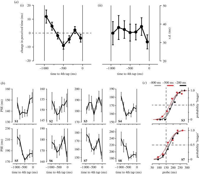
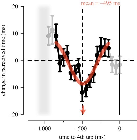
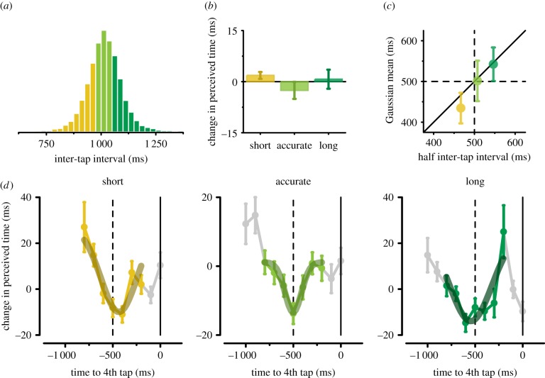
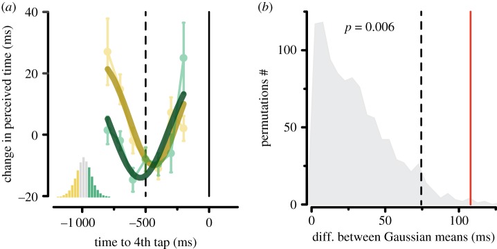
Temporal processing is fundamental for an accurate synchronization between motor behaviour and sensory processing. Here, we investigate how motor timing during rhythmic tapping influences perception of visual time. Participants listen to a sequence of four auditory tones played at 1 Hz and continue the sequence (without auditory stimulation) by tapping four times with their finger. During finger tapping, they are presented with an empty visual interval and are asked to judge its length compared to a previously internalized interval of 150 ms. The visual temporal estimates show non-monotonic changes locked to the finger tapping: perceived time is maximally expanded at halftime between the two consecutive finger taps, and maximally compressed near tap onsets. Importantly, the temporal dynamics of the perceptual time distortion scales linearly with the timing of the motor tapping, with maximal expansion always being anchored to the centre of the inter-tap interval. These results reveal an intrinsic coupling between distortion of perceptual time and production of self-timed motor rhythms, suggesting the existence of a timing mechanism that keeps perception and action accurately synchronized.

Keywords: action–perception coupling; finger tapping; sensorimotor; time perception; timing.

Figure 1.

Experimental set-up and procedure. (a) Participants sat in front of a table where two LEDs were positioned, one providing the fixation point (FIX. LED, red) and the other delivering the visual stimulus (STIM. LED, yellow). Participants kept their right index finger on a small button laying on a rigid support below the table. The auditory tones were delivered by two loudspeakers placed in front of the participants. (b) Trial started with the FIX. LED being lit. Four auditory tones (800 Hz, 50 ms) were then played at 1 Hz (inter-sound interval: 1 000 ms; marked in blue). Participants were asked to continue the sequence of tones by pressing the button four times with their right index finger at the same rate as the sound presentation. At random times between the 3rd and the 4th button press (marked in orange), two visual flashes (5 ms each) were presented separated by a variable temporal interval centred on 150 ms (probe; marked in yellow). Participants were required to report verbally whether the probe interval was shorter or longer compared with the standard interval (150 ms, presented at the beginning of each block; not shown).

Figure 2.

(a) (i) Average perceived duration (expressed as deviation from the mean PSE; see Methods) as a function of stimulus latency (time zero: 4th finger tap onset). Positive values indicate (relative) compression of time, negative values indicate (relative) expansion of time. The dashed horizontal line indicates no (relative) change in perceived duration. Solid vertical lines at −1 000, −500, and 0 ms: beginning, centre, and end of the instructed inter-tap interval (1 000 ms), respectively. Error bars represent s.e.m. (ii) Average (inverse) of the precision of the temporal judgements (s.d.) plotted as a function of stimulus latency (relative to 4th tap onset). Error bars represent s.e.m. (b) Individual PSEs as a function of stimulus latency. (c) Psychometric functions showing the proportion of trials where the probe interval was perceived as longer than the standard interval (150 ms; dashed vertical line). Results for two representative subjects (S3 and S7) are shown separately for probe intervals presented at −800 ms (light grey), −500 ms (red), and −200 ms (black) relative to 4th tap onset. Dots represent binned data points.

Figure 3.

Change in the perceived duration (relative to the PSE estimated on the entire set of trials) aligned to the 4th tap and calculated on the data pooled across subjects. Error bars represent standard errors (s.e.) estimated by bootstrap. The Gaussian function that best fits the data in the range from −850 to −150 ms (black symbols) is plotted in red. Red arrow: mean of the best-fitting Gaussian function (−495 ms, indexing the latency of maximal time expansion). Grey shaded area: onset of the 3rd finger tap (mean ± 1 s.d.).

Figure 4.

(a) Distribution of the (last) inter-tap interval (data pooled across subjects). Trials are split into three categories: (i) short inter-taps (0.25 quantile of the distribution, yellow), (ii) accurate inter-taps (between the 0.35 and the 0.65 quantile, light green), and (iii) long inter-taps (≥0.75 quantile, dark green). (b) Average perceived duration (expressed as deviation from the mean PSE) for the short, accurate, and long trial categories (data collapsed across stimulus latencies). Error bars represent s.e.m. (c) The mean of the best-fitting Gaussian function is plotted against half of the inter-tap interval (median values) for the short (yellow), accurate (light green), and long (dark green) categories of trials. Error bars represent 90% confidence intervals calculated by bootstrap. The diagonal indicates that maximal perceived time expansion occurs halfway between the two consecutive finger taps. (d) Perceived visual duration aligned with the 4th tap and best-fitting Gaussian functions for the short, accurate, and long trials. Coloured symbols indicate the data used to fit the Gaussian functions (i.e. from −800 to −200 ms); data marked in grey were not used for the Gaussian modelling. Error bars represent s.e. estimated by bootstrap.

Figure 5.

(a) Best-fitting Gaussian functions for the short (yellow) and long (dark green) inter-tap categories superimposed to the time courses in perceived duration aligned to the 4th tap (same data shown in figure 4d). (b) Distribution of the difference between the means of the best-fitting Gaussian functions (indexing the latencies of maximal time expansion) obtained by randomly permuting (1 000 iterations) the trials belonging to the short and to the long categories. Dashed line: 0.95 quantile of the distribution. Red line: difference between the means of the Gaussian functions fitted to the short and long inter-tap trials.

References

1. Mauk MD, Buonomano DV. 2004. The neural basis of temporal processing. Annu. Rev. Neurosci. 27, 307–340. (10.1146/annurev.neuro.27.070203.144247) - DOI - PubMed
1. Wiener M, Turkeltaub P, Coslett HB. 2010. The image of time: a voxel-wise meta-analysis. Neuroimage 49, 1728–1740. (10.1016/j.neuroimage.2009.09.064) - DOI - PubMed
1. Buhusi CV, Meck WH. 2005. What makes us tick? Functional, neural mechanisms of interval timing. Nat. Rev. Neurosci. 6, 755–765. (10.1038/nrn1764) - DOI - PubMed
1. Ivry RB, Spencer RM. 2004. The neural representation of time. Curr. Opin Neurobiol. 14, 225–232. (10.1016/j.conb.2004.03.013) - DOI - PubMed
1. Merchant H, Yarrow K. 2016. How the motor system both encodes and influences our sense of time. Curr. Opin. Behav. Sci. 8, 22–27. (10.1016/j.cobeha.2016.01.006) - DOI
Publication types