Color statistics of objects, and color tuning of object cortex in macaque monkey

Abstract

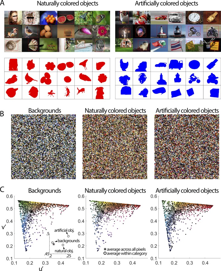
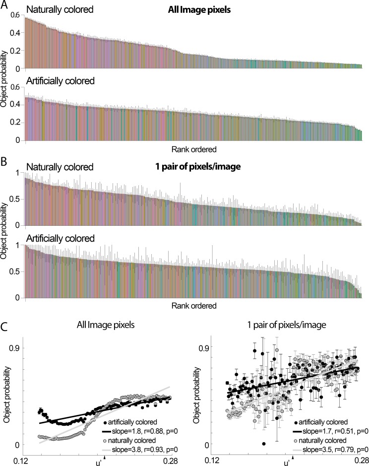
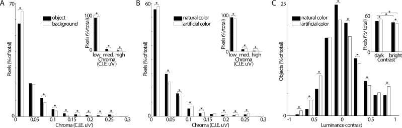
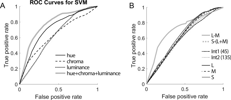
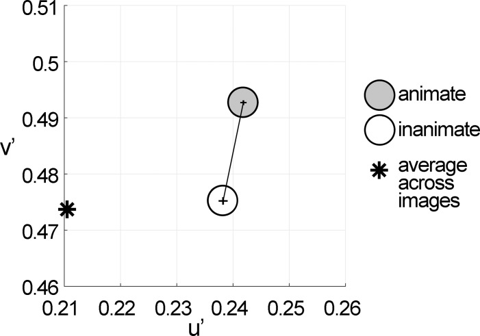
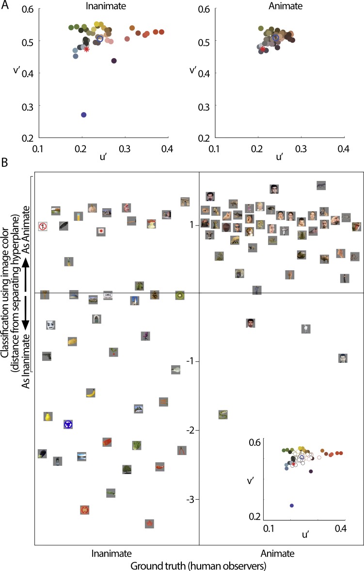
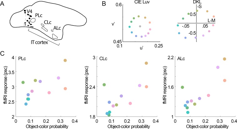
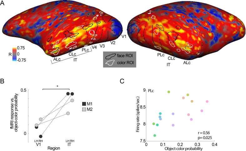
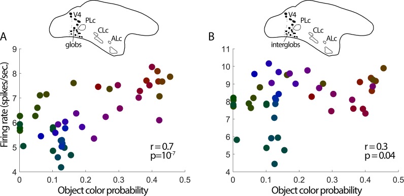
We hypothesized that the parts of scenes identified by human observers as "objects" show distinct color properties from backgrounds, and that the brain uses this information towards object recognition. To test this hypothesis, we examined the color statistics of naturally and artificially colored objects and backgrounds in a database of over 20,000 images annotated with object labels. Objects tended to be warmer colored (L-cone response > M-cone response) and more saturated compared to backgrounds. That the distinguishing chromatic property of objects was defined mostly by the L-M post-receptoral mechanism, rather than the S mechanism, is consistent with the idea that trichromatic color vision evolved in response to a selective pressure to identify objects. We also show that classifiers trained using only color information could distinguish animate versus inanimate objects, and at a performance level that was comparable to classification using shape features. Animate/inanimate is considered a fundamental superordinate category distinction, previously thought to be computed by the brain using only shape information. Our results show that color could contribute to animate/inanimate, and likely other, object-category assignments. Finally, color-tuning measured in two macaque monkeys with functional magnetic resonance imaging (fMRI), and confirmed by fMRI-guided microelectrode recording, supports the idea that responsiveness to color reflects the global functional organization of inferior temporal cortex, the brain region implicated in object vision. More strongly in IT than in V1, colors associated with objects elicited higher responses than colors less often associated with objects.

Figure 1

The color statistics of objects. (A) From over 200,000 images, observers at Microsoft selected 20,840 images that contained a salient object and placed a red bounding box around the object (Liu et al., 2007). Two naïve observers in the present study then created masks to demarcate the pixels containing the object. The top panels show example images; the bottom panels show the masks. Images from the MRSA database (Liu et al., 2007) are reproduced with permission from Microsoft. (B) Tapestry plots showing 10,000 pixels randomly selected from the pixels assigned to backgrounds (1.89 billon pixels total), naturally colored objects (0.26 billion pixels), and artificially colored objects (0.22 billion pixels). (C) Chromaticity coordinates of the pixel colors of the tapestry plots. The figure shows a single lightness plane through the chromaticity space, with pixels of all lightness projected onto that plane. The lightness values are indicated by the colors of the data points. Inset shows an expanded view. The symbols contain the standard error of the mean. The analysis was repeated 100 times; each iteration involved randomly sampling 10,000 pixels of backgrounds, artificially colored objects, and naturally colored objects. Pixels from naturally colored objects were different from pixels in backgrounds along the u′ dimension (p = 0 for all 100 iterations, unpaired t test), and along the v′ direction (p < 10⁻⁶⁷ for all 100 iterations). Pixels from artificially colored objects were different from pixels in backgrounds along the u′ dimension (p < 10⁻⁸² for all 100 iterations), and along the v′ direction (p < 0.05 for 76/100 iterations). Pixels from artificially colored objects were different from pixels in naturally colored objects along the u′ dimension (p < 10⁻²⁶ for all 100 iterations), and along the v′ direction (p < 10⁻¹³⁰ for all 100 iterations).

Figure 2

Object-color probability, rank-ordered by most frequent object colors. (A) Pixels across the 20,840 images were categorized into 240 bins (24 evenly spaced hue angles at 10 chroma values in u′ v′). Object-color probability was computed as follows: number of pixels having a given color in the objects divided by the number of pixels having the same color in the objects + backgrounds. The colors of the bars correspond to the sRGB colors of the bins. The bars are rank-ordered with the most frequently occurring object colors on the left. The error bars show the standard deviation of the probability of a given hue being in the foreground, computed over 1000 bootstraps (bar height is the mean of the bootstrapped values). During each bootstrap, 20000 images were picked randomly to generate probabilities. The results across bootstraps were averaged together to generate mean object-background probabilities (bar height); (B) as for panel (A), but using for each image only one randomly selected pixel for each object and one randomly selected pixel for each background. (C) Correlation of object-color probability as a function of u′, for all pixels (left) and single pairs of pixels per image (right). The colors were binned in 101 bins (0.0014 u′ bin widths), evenly sampling the u′ values symmetric over the white point (arrowhead); error bars show standard deviations, computed as in panel A.

Figure 3

Color chroma and luminance-contrast statistics of objects. (A) Histograms showing the chroma of the pixels identified as part of objects (black bars), and the chroma of the pixels identified as part of backgrounds (open bars; same data sampling as in Figure 2B). Chroma was defined as the CIE 1976 chroma. Insets bin chroma values 0–0.10 as “low,” 0.11–0.20 as “medium,” and 0.01–0.30 as “high”. (B) The chroma of pixels identified as naturally colored (black bars) and artificially colored (open bars). Artificially colored objects were biased towards the chroma extremes, showing more low-chroma pixels and more high-chroma pixels compared to naturally colored objects (this observation is not apparent when chroma values are binned more coarsely, as shown in the inset). Other conventions as in panel (A). (C) The luminance contrast of all image pixels identified as part of naturally colored objects (black bars) are compared against the contrast of the pixels identified as part of artificially colored objects (white bars). Michelson contrast was computed by taking, for each image, the average luminance across the pixels of the object minus the average luminance of the pixels in the background divided by the sum of these luminance values. Insets bin luminance contrast values −1 to 0 as “dark,” and 0 to 1 as “bright”. All differences between pairs of bars identified by an asterisk were significant (chi-square test of proportions, p < 0.03).

Figure 4

Receiver operating characteristic (ROC) analysis showed that objects can be discriminated from backgrounds based on color. (A) ROC curves when using hue, chroma, and luminance, and all three as input to a support vector machine (SVM) classifier. All ROC curves were significantly different from the null curve (Wilcoxon rank sum test, p < 0.0001). (B) ROC curves when using L, M, S, L-M, S−(L-M), and the two intermediate directions in cone-opponent space as features for SVM for classification (Int1 = orange-blue axis; Int2 = green-purple axis). All ROC curves were different from the null curve (Wilcoxon rank sum test, p < 0.0001). Only the L-M curve and the S curve were different from all other curves, and each other (p < 0.0001).

Figure 5

Color statistics differed for animate and inanimate objects. Average chromaticity coordinates for pixels identified as part of animate or inanimate objects. Pixels were drawn from a tapestry of 10,000 randomly selected pixels from each category. This analysis was repeated 100 times (see Figure 2C). Pixels of animate objects were different from pixels of inanimate objects along the u′ dimension (p < 0.05 for 77/100 iterations), and along the v′ direction (p < 10⁻⁸⁰ for all 100 iterations). Error bars are SEM.

Figure 6

Images could be categorized as animate versus inanimate using only the average color of the object in each image. (A) Chromaticity coordinates for the 92 images used by Kriegestkorte et al. (2008). The asterisks show the neutral point of the color space. The blue circles are the average u′ v′ value of all the color values plotted in the figure. (B) A support vector machine with a radial basis function trained on only the average CIE u′ v′ of the object in each image categorized animate images at an accuracy of 91.67% and inanimate images at an accuracy of 70.45%. Inset shows the chromaticity coordinates for all images as in A, in which open symbols indicate images classified as “animate” and filled symbols indicated images classified as “inanimate”. Stimuli are reproduced with permission from Nico Kriegeskorte.

Figure 7

Correlation of object-color statistics and color-tuning of IT color-biased regions. A. Diagram of the lateral view of the macaque brain showing the location of the color-biased regions in inferior temporal cortex (IT), anterior is to the right (Posterior Lateral color, PLc; Central Lateral color, CLc; and Anterior lateral color, ALc; Lafer-Sousa & Conway, 2013). (B) Chromaticities of the colors used in these fMRI experiments. (C) Relationship of the probability of object colors versus color-tuning of color-biased regions within IT. Object-color probability was computed as follows: number of pixels having a given color in the objects divided by the number of pixels having the same color in the objects + background, in natural images. All three regions showed higher responses for colors that were more likely to be the colors of objects (PLc: r = 0.7, p = 0.01; CLc: r = 0.72, p = 0.01; ALc: r = 0.65, p = 0.03). fMRI response (psc) = percent signal change (measured against the signal measured for gray blocks between each colored block).

Figure 8

Correlation of object-color statistics across the cerebral cortex. (A) Correlation coefficients between fMRI color tuning and object-color probabilities assessed for each voxel across both hemispheres for one monkey (M1). Color-biased regions are outlined in white; face patches are outlined in black. Vertical meridians are shown as broken lines; horizontal meridians are shown as solid lines. (B) Correlation coefficients were higher in IT compared to V1; the IT region of interest was defined by combining the color-biased regions and the face patches (paired t test across V1 and IT, p = 0.03; LH = left hemisphere; RH = right hemisphere). (C) The population of neurons recorded in fMRI-guided recordings of the posterior color-biased region showed a bias for colors more often associated with objects, consistent with the fMRI results (r = 0.56, p = 0.025). Data were obtained from 117 cells in 54 penetrations in M1.

Figure 9

Color-tuning of the population of neurons recorded in posterior IT (the V4 Complex) was correlated with object-color statistics. (A) Responses of cells located within globs (fMRI-identified color-biased regions of the V4 Complex; N = 300 cells. The glob-cell population showed a stronger response to the colors more likely associated with naturally colored objects (r = 0.7, p = 10⁻⁰⁷). (B) Responses of cells located within interglob regions (N = 181 cells). The interglob-cell population showed a stronger response to the colors more likely associated with objects, but a lower correlation coefficient than was found among glob cells (r = 0.3, p = 0.04, Fisher z′ = 2.2, p = 0.02).

References

1. Bartels A, Zeki S. The architecture of the colour centre in the human visual brain: New results and a review. The European Journal of Neuroscience. (2000);12(1):172–193. - PubMed
1. Beauchamp M. S, Haxby J. V, Jennings J. E, DeYoe E. A. An fMRI version of the Farnsworth-Munsell 100-Hue test reveals multiple color-selective areas in human ventral occipitotemporal cortex. Cerebral Cortex. (1999);9(3):257–263. - PubMed
1. Bohon K. S, Hermann K. L, Hansen T, Conway B. R. Representation of perceptual color space in macaque posterior inferior temporal cortex (the V4 complex) eNeuro. (2016);3(4):1–28.:e0039–16.2016. - PMC - PubMed
1. Caramazza A, Shelton J. R. Domain-specific knowledge systems in the brain: The animate-inanimate distinction. Journal of Cognitive Neuroscience. (1998);10(1):1–34. - PubMed
1. Chang C.-C, Lin C.-J. LIBSVM : A library for support vector machines. ACM Transactions on Intelligent Systems and Technology. (2011);2(27):1–27. http://www.csie.ntu.edu.tw/∼cjlin/libsvm.
Publication types