The value of using seasonality and meteorological variables to model intra-urban PM2.5 variation

Abstract

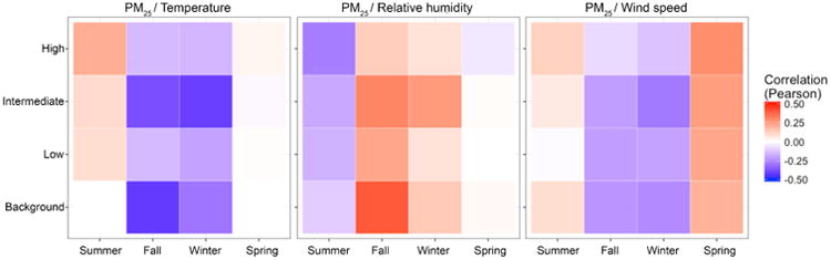
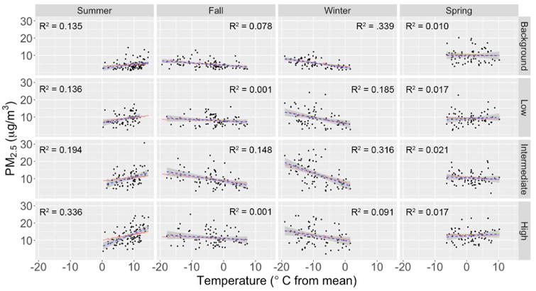
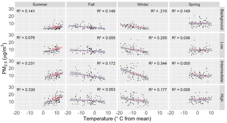
A yearlong air monitoring campaign was conducted to assess the impact of local temperature, relative humidity, and wind speed on the temporal and spatial variability of PM_2.5 in El Paso, Texas. Monitoring was conducted at four sites purposely selected to capture the local traffic variability. Effects of meteorological events on seasonal PM_2.5 variability were identified. For instance, in winter low-wind and low-temperature conditions were associated with high PM_2.5 events that contributed to elevated seasonal PM_2.5 levels. Similarly, in spring, high PM_2.5 events were associated with high-wind and low-relative humidity conditions. Correlation coefficients between meteorological variables and PM_2.5 fluctuated drastically across seasons. Specifically, it was observed that for most sites correlations between PM_2.5 and meteorological variables either changed from positive to negative or dissolved depending on the season. Overall, the results suggest that mixed effects analysis with season and site as fixed factors and meteorological variables as covariates could increase the explanatory value of LUR models for PM_2.5.

Keywords: Temperature; air pollution; land use regression; relative humidity; wind speed.

Figure 1

Hourly averaged PM_2.5 concentrations plotted as a function of wind speed by season. The color scale represents temperature values and the circle size represents relative humidity values. Also shown in each panel are seasonal averages for each variable represented in the plot. USE COLOR IN PRINT

Figure 2

Diurnal variation of hourly averaged PM_2.5 concentrations by site during the study period (A) and by season (B). Also, shown in each panel is the corresponding coefficient of variation (CV) for PM₂.₅ observations across all sites. USE COLOR IN PRINT

Figure 3

Correlation panels with fill color representing Pearson correlation coefficient values. The corresponding p-values for the Pearson correlation coefficients are provided in Table S3. USE COLOR IN PRINT

Figure 4

Scatter plots for temperature and PM_2.5. Also shown are empirical R² values as well as PM_2.5 values (solid red line) estimated with a mixed effects model for PM_2.5 across the study region with Site and Season as factors, a constant slope for relative humidity, and random slopes for temperature across sites and seasons. The small variation in the estimated PM_2.5 values was caused by variation in relative humidity. To serve as reference the dashed blue line was fitted by panel via a standard linear regression between PM_2.5 with the standard error represented by the shaded area. Temperature values have been centered to the study average. DO NOT USE COLOR IN PRINT

Figure 5

Scatter plots for temperature and PM_2.5. Also shown are Pseudo R² values as well as PM_2.5 values (solid red line) estimated with a mixed effects model for PM_2.5 across the study region with Site and Season as factors, constant slopes for cosinor terms( $sin\frac{2\pi \mathit{\text{Day}}}{365}$, $sin\frac{2\pi \mathit{\text{Day}}}{180}$, $cos\frac{2\pi \mathit{\text{Day}}}{365}$, $cos\frac{2\pi \mathit{\text{Day}}}{180}$)) and random slopes or temperature across sites and seasons. The small variation in the estimated PM_2.5 values was caused by variation in the cosinor terms. To serve as reference the dashed blue line was fitted by panel via a standard linear regression between PM_2.5 with the standard error represented by the shaded area. Temperature values have been centered to the study average. DO NOT USE COLOR IN PRINT

References

1. Arain MA, Blair R, Finkelstein N, Brook JR, Sahsuvaroglu T, Beckerman B, Zhang L, Jerrett M. The use of wind fields in a land use regression model to predict air pollution concentrations for health exposure studies. 2007;41:3453–3464. doi: 10.1016/j.atmosenv.2006.11.063. - DOI
1. Armijos RX, Weigel MM, Myers OB, Li WW, Racines M, Berwick M. Residential Exposure to Urban Traffic Is Associated with Increased Carotid Intima-Media Thickness in Children 1 –11. 2015 doi: 10.1155/2015/713540. - DOI - PMC - PubMed
1. Both AF, Westerdahl D, Fruin S, Haryanto B, Marshall JD. Exposure to carbon monoxide, fine particle mass, and ultrafine particle number in Jakarta, Indonesia: Effect of commute mode. Science of the Total Environment, The. 2013;443:965–972. doi: 10.1016/j.scitotenv.2012.10.082. - DOI - PubMed
1. Briggs D. The role of GIS: coping with space (and time) in air pollution exposure assessment. J Toxicol Environ Health Part A. 2005;68:1243–1261. doi: 10.1080/15287390590936094. - DOI - PubMed
1. Briggs D, Collins S, Elliott P, Fischer P, Kingham S, Lebret E, Pryl K, Van Reeuwijk H, Smallbone K, Van der Veen A. Mapping urban air pollution using GIS: A regression-based approach. International Journal of Geographical Information Science. 1997;11:699–718.
LinkOut - more resources